Hooke's Law Spring Force Solver ($F = -kx$)

1. Introduction

Why does a mechanical wristwatch continue ticking with atomic-like precision for years without electrical batteries? Why do modern automotive suspension systems glide seamlessly over rough road potholes and speed bumps? Why does an archer's drawn composite bow store lethal kinetic work waiting to propel an arrow hundreds of meters?

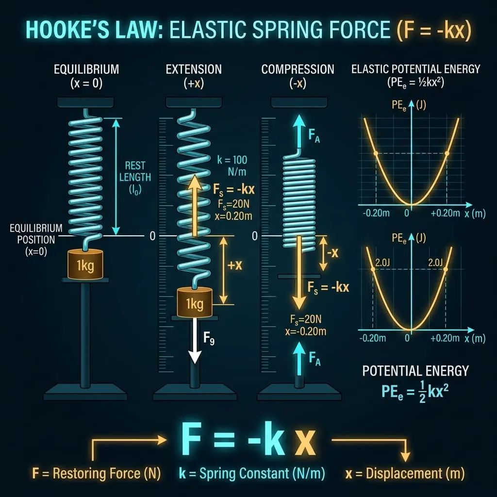
At the foundational bedrock of all structural mechanics, mechanical engineering, materials science, and vibrational physics lies a single, elegant governing principle: Hooke's Law ($F = -kx$).

Formulated in 1676 by English polymath Robert Hooke under the Latin anagram "ceiiinosssttuv" (decoded in 1678 as "Ut tensio, sic vis" — "As the extension, so the force"), Hooke's Law describes the linear proportional relationship between the force applied to deform an elastic body and the resulting displacement or strain produced.

graph LR
    K["🌀 Spring Constant (k)
Stiffness in N/m"] --> MULT["✖️ Multiplied By"]
    X["📏 Displacement (x)
Stretch / Compression in Meters (m)"] --> MULT
    MULT --> F["💥 Restoring Force (F)
F = -kx in Newtons (N)"]
    F --> E["⚡ Elastic Potential Energy
U_s = ½ · k · x² (Joules)"]
    F --> SHM["🔄 Simple Harmonic Motion
Period: T = 2π √(m / k)"]

Mastering Hooke's Law and elastic mechanics enables engineers, roboticists, and physicists to: - Design vehicle suspension coil springs, anti-roll torsion bars, and pneumatic dampers that optimize passenger comfort and tire road contact. - Calibrate industrial load cells, piezoelectric force transducers, and precision mechanical spring scales. - Engineer earthquake base isolation dampers and tuned mass dampers that protect skyscrapers from seismic resonant destruction. - Calculate atomic bond vibrational frequencies in infrared molecular spectroscopy. - Model biological soft tissue biomechanics, such as tendon elasticity and cardiovascular arterial wall compliance.

2. Definitions & Analogies

2.1 The Simple Definition

In simple everyday terms: - Displacement ($x$) is "how much you stretch or compress a spring" away from its natural resting position. - Spring Constant ($k$) is "how stiff the spring is" (measured in Newtons per meter, $\text{N/m}$). A soft mattress spring has a small $k$; a heavy truck leaf spring has an immense $k$. - Restoring Force ($F$) is "how hard the spring fights back" to return to its original length. - Hooke's Law states that if you double the stretch distance, the spring pulls back with twice as much force. If you push or pull in one direction ($+x$), the spring pushes back in the exact opposite direction ($-F$), which is why the equation contains a negative sign.

2.2 The Formal Technical Definition

Scalar & Vector Formulations

For an ideal linear elastic spring deformed within its proportional limit:

Where: - $F_{\text{restoring}}$ is the elastic restoring force exerted by the spring ($\text{Newtons, N}$). - $k$ is the spring constant (stiffness factor) in Newtons per meter ($\text{N/m}$ or $\text{kg/s}^2$). - $x = L - L_0$ is the displacement vector from the unstretched resting equilibrium length ($L_0$) in meters ($\text{m}$). - The negative sign ($-$) indicates that the restoring force is always directed opposite to the displacement vector, pulling toward the equilibrium position ($x = 0$).

Elastic Potential Energy ($U_s$ or $PE_{\text{elastic}}$)

Because the restoring force increases linearly with displacement ($F(x) = kx$), the mechanical work ($W$) performed to stretch or compress a spring from $x = 0$ to displacement $x$ is obtained by integration:

• SI Unit: Joule ($\text{J}$) $\equiv \text{N}\cdot\text{m} \equiv \text{kg}\cdot\text{m}^2/\text{s}^2$.

2.3 The Trampoline / Rubber Band Analogy

To visualize Hooke's Law intuitively, consider jumping on a heavy recreational trampoline:

graph TD
    subgraph Trampoline_Analogy ["🤸 Trampoline Surface Analogy"]
        Standing["Gentle Stand (x = 0.05 m)
Low Displacement → Mild Upward Push (F = -kx)"]
        DeepJump["High Jump Impact (x = 0.50 m)
10× Displacement → 10× Fiercer Upward Push"]
        StoredEnergy["Elastic Energy Scales with x²
10× Depth → 100× Stored Rebound Work (½kx²)"]
        Standing --> DeepJump --> StoredEnergy
    end

1. Light Step: When you gently step onto the trampoline canvas, it deflects downward by a few centimeters, providing a mild upward support force.
2. Deep Bounce: When you leap high and land forcefully, the canvas deflects downward $10\times$ deeper. The springs pull back with $10\times$ more force, and store $100\times$ ($10^2$) more elastic potential energy, catapulting you high into the air on the rebound!

3. History & Milestones in Elasticity Theory

timeline
    title Milestones in Hooke's Law & Continuum Elasticity
    1676 : Robert Hooke conceives the law of elasticity as Latin anagram 'ceiiinosssttuv'
    1678 : Hooke publishes 'De Potentia Restitutiva' ('Ut tensio, sic vis')
    1705 : Jacob Bernoulli analyzes bending beams and flexible elastica curves
    1744 : Leonhard Euler formulates the column buckling stability equation
    1807 : Thomas Young defines the fundamental modulus of elasticity (Young's Modulus E)
    1822 : Augustin-Louis Cauchy establishes the 3D stress and strain tensor formulations

• Robert Hooke's Discovery (1676): English polymath Robert Hooke invented the balance spring for pocket watches, which replaced unwieldy gravity pendulums and revolutionized maritime navigation. Hooke realized that all solid bodies—whether metal spirals, wooden beams, or glass fibers—exhibit linear proportional deformation under moderate loads.
• Thomas Young & Young's Modulus ($E$, 1807): British polymath Thomas Young generalized Hooke's 1D spring law into an intrinsic intensive material property, defining Young's Modulus ($E$) as the ratio of tensile stress ($\sigma$) to tensile strain ($\varepsilon$), allowing engineers to predict stiffness for any material geometry.
• Cauchy's 3D Continuum Mechanics (1822): French mathematician Augustin-Louis Cauchy expanded Hooke's 1D equation into the generalized 3D tensor formulation of linear elasticity ($\sigma_{ij} = C_{ijkl} \varepsilon_{kl}$), governing modern finite element structural engineering analysis.

4. Stress, Strain, and the Complete Tensile Curve

In materials science and mechanical design, Hooke's Law is valid only within a specific material loading zone known as the Proportional Linear Elastic Region:

graph LR
    A["0: Rest / Origin"] -->|"Hooke's Law Holds (σ = E·ε)"| B["A: Proportional Limit"]
    B --> C["B: Elastic Yield Point (σ_y)"]
    C -->|"Plastic Permanent Deformation"| D["C: Ultimate Tensile Strength (UTS)"]
    D -->|"Necking"| E["D: Fracture / Rupture Point"]

5. Springs in Series and Parallel Configurations

When multiple springs are combined in mechanical assemblies, their effective composite spring constant ($k_{\text{eq}}$) depends strictly on their geometric connection topology:

graph TD
    COMBO["🌀 Multi-Spring Systems"] --> PAR["🟢 Springs in Parallel"]
    COMBO --> SER["🔵 Springs in Series"]
    
    PAR -->|"Formulation"| P_FORM["• Identical Displacement: x₁ = x₂ = x
• Forces Add: F_total = F₁ + F₂
• Equivalent Constant: k_eq = k₁ + k₂ + k₃ + ...
• Result: STIFFNESS INCREASES"]
    
    SER -->|"Formulation"| S_FORM["• Identical Force: F₁ = F₂ = F
• Displacements Add: x_total = x₁ + x₂
• Equivalent Constant: 1/k_eq = 1/k₁ + 1/k₂ + ...
• Result: STIFFNESS DECREASES (Softer)"]

6. Simple Harmonic Motion (SHM) Dynamics

An ideal mass ($m$) attached to a spring of constant ($k$) oscillating on a frictionless horizontal surface performs Simple Harmonic Motion (SHM) governed by Newton's Second Law:

• Natural Angular Frequency ($\omega_0$): $\omega_0 = \sqrt{\frac{k}{m}} \quad (\text{rad/s})$

• Natural Oscillation Frequency ($f$): $f = \frac{\omega_0}{2\pi} = \frac{1}{2\pi} \sqrt{\frac{k}{m}} \quad (\text{Hertz, Hz})$

• Natural Period of Oscillation ($T$): $T = \frac{1}{f} = 2\pi \sqrt{\frac{m}{k}} \quad (\text{Seconds, s})$

7. Master Formula Matrix & Step-by-Step Problem Solver

8. Practical Real-World Calculation Examples

Example 1: Vehicle Suspension Corner Spring Deflection

- Scenario: A passenger car corner carries a static corner curb weight of $m = 400.0\text{ kg}$. The suspension coil spring has a stiffness constant $k = 32,000\text{ N/m}$. - Step 1: Calculate Downward Gravitational Force: $F_g = m \cdot g = 400.0\text{ kg} \times 9.80665\text{ m/s}^2 = 3,922.66\text{ Newtons}$

• Step 2: Calculate Static Compression Displacement ($x$): $x = \frac{F}{k} = \frac{3,922.66\text{ N}}{32,000\text{ N/m}} \approx \mathbf{0.1226\text{ meters}} = \mathbf{12.26\text{ cm}} \quad (\approx 4.83\text{ inches})$

• Step 3: Calculate Stored Elastic Energy ($U_s$): $U_s = \frac{1}{2} k x^2 = 0.5 \times 32,000 \times (0.1226)^2 \approx \mathbf{240.47\text{ Joules}}$

Example 2: Bungee Jumping Elastic Cord Sizing

- Scenario: An $80.0\text{ kg}$ jumper leaps from a high bridge using a bungee cord of resting length $L_0 = 30.0\text{ m}$ with a spring constant $k = 40.0\text{ N/m}$. - Maximum Cord Stretch ($x_{\max}$) via Energy Conservation ($mgh = \frac{1}{2}kx^2$): $m g (L_0 + x) = \frac{1}{2} k x^2 \implies (80.0)(9.81)(30.0 + x) = 0.5(40.0) x^2$ $23,544 + 784.8 x = 20.0 x^2 \implies 20 x^2 - 784.8 x - 23,544 = 0$ $x^2 - 39.24 x - 1,177.2 = 0 \implies x_{\max} = \frac{39.24 + \sqrt{(-39.24)^2 - 4(1)(-1,177.2)}}{2} \approx \mathbf{58.82\text{ meters}}$

• Peak Deceleration Force Felt by Jumper: $F_{\max} = k \cdot x_{\max} = 40.0\text{ N/m} \times 58.82\text{ m} = \mathbf{2,352.8\text{ Newtons}} \quad (\approx 3.0\text{ Gs, safe})$

Example 3: Precision Laboratory Spring Scale Calibration

- Scenario: A precision analytical spring scale extends by $x = 15.0\text{ mm} = 0.0150\text{ m}$ when a standard calibration mass of $m = 300.0\text{ grams} = 0.300\text{ kg}$ is suspended. - Calculated Spring Constant ($k$): $F = m \cdot g = 0.300\text{ kg} \times 9.80665\text{ m/s}^2 = 2.942\text{ Newtons}$ $k = \frac{F}{x} = \frac{2.942\text{ N}}{0.0150\text{ m}} = \mathbf{196.13\text{ N/m}}$

Example 4: Archery Compound Bow Energy Storage & Arrow Launch Speed

- Scenario: A modern compound hunting bow behaves like an effective spring with $k = 1,400\text{ N/m}$ drawn back by $x = 0.50\text{ meters}$ ($50\text{ cm}$). It fires a lightweight carbon arrow of mass $m = 0.025\text{ kg}$ (25 grams). - Stored Elastic Potential Energy: $U_s = \frac{1}{2} k x^2 = 0.5 \times 1,400 \times (0.50)^2 = 700 \times 0.25 = \mathbf{175.0\text{ Joules}}$

• Theoretical Arrow Velocity ($v = \sqrt{2U_s / m}$, assuming $85\%$ mechanical efficiency): $KE_{\text{arrow}} = 175.0\text{ J} \times 0.85 = 148.75\text{ J}$ $v = \sqrt{\frac{2 \times 148.75\text{ J}}{0.025\text{ kg}}} = \sqrt{11,900} \approx \mathbf{109.09\text{ m/s}} \quad (\approx 392.7\text{ km/h} \approx 244\text{ mph})$

Example 5: Springs in Series vs. Parallel Equivalent Stiffness

- Scenario: Two identical suspension springs each have a spring constant $k_1 = k_2 = 500\text{ N/m}$. - Parallel Configuration ($k_{\text{parallel}}$): $k_{\text{parallel}} = k_1 + k_2 = 500 + 500 = \mathbf{1,000\text{ N/m}} \quad (\text{Twice as stiff})$

• Series Configuration ($k_{\text{series}}$): $k_{\text{series}} = \frac{k_1 k_2}{k_1 + k_2} = \frac{500 \times 500}{500 + 500} = \frac{250,000}{1,000} = \mathbf{250\text{ N/m}} \quad (\text{Half as stiff / twice as soft})$

9. Real-World Engineering Case Studies

Case Study 1: Tuned Mass Dampers (TMD) in Megatall Skyscrapers (Taipei 101)

- Engineering Dilemma: The $508\text{ meter}$ tall Taipei 101 skyscraper in Taiwan is subjected to violent typhoon winds ($>200\text{ km/h}$) and frequent tectonic earthquakes. Uncontrolled wind vortex shedding can sway the building's apex by over $1.5\text{ meters}$, inducing structural fatigue and passenger motion sickness. - TMD Solution Physics: Engineers suspended a massive steel sphere of mass $M = 660,000\text{ kg}$ (660 metric tons) on the 88th floor, supported by eight heavy hydraulic spring-damper assemblies. - Tuning Frequency: The natural frequency of the building's fundamental sway mode is $f_{\text{building}} \approx 0.15\text{ Hz}$ ($T \approx 6.7\text{ seconds}$). - Calculated Required Spring Constant ($k$): $\omega_0 = 2\pi f = 2\pi (0.15) \approx 0.9425\text{ rad/s}$ $k = M \cdot \omega_0^2 = 660,000\text{ kg} \times (0.9425)^2 \approx 660,000 \times 0.8883 \approx \mathbf{586,278\text{ N/m}} \quad (\approx 586.3\text{ kN/m})$

• Dynamic Result: When typhoon winds push the skyscraper to the left, the heavy pendulum swings to the right ($180^\circ$ out of phase), transmitting counteracting Hookean restoring forces that dissipate over $40\%$ of the building's sway energy, keeping the tower structurally safe and comfortable.

Case Study 2: Geotechnical Earthquake Base Isolation Rubber Bearings

- Building Safety Challenge: In high-risk seismic zones (like San Francisco or Tokyo), hospital foundations must survive catastrophic ground accelerations during magnitude $8.0+$ earthquakes without structural column collapse. - Engineering Design: Elastomeric Lead-Rubber Bearings (LRB) consisting of alternating layers of vulcanized rubber sheets and steel shims are installed under the building's foundation columns. - Mechanical Operation: - Vertically, the layered steel shims provide ultra-high stiffness ($k_v > 10^9\text{ N/m}$) to support the massive multi-story building weight. - Horizontally, the rubber layers provide low lateral shear stiffness ($k_h \approx 1.2 \times 10^6\text{ N/m}$), lengthening the natural vibration period from $T = 0.4\text{ s} \to 2.5\text{ s}$. - Performance: Because earthquake ground shaking energy is concentrated at high frequencies ($2\text{–}5\text{ Hz}$), softening the lateral stiffness through Hookean rubber shear decouples the building from the vibrating ground, reducing peak horizontal accelerations transmitted to the hospital floors by over $75\%$.

10. Common Mistakes & How to Avoid Them

11. Frequently Asked Questions (FAQ)

Q1: Why does Hooke's Law have a negative sign ($-kx$)?

A: The negative sign signifies that the spring's internal restoring force is always directed in the exact opposite direction of the displacement vector. If you displace the spring to the right ($+x$), the restoring force pulls to the left ($-F$); if you compress to the left ($-x$), the restoring force pushes back to the right ($+F$).

Q2: What is the physical meaning of the spring constant ($k$)?

A: The spring constant ($k$) measures the intrinsic mechanical stiffness of the spring. A value of $k = 500\text{ N/m}$ means it requires $500\text{ Newtons}$ of applied force ($\approx 51\text{ kg}$ of weight) to stretch or compress the spring by exactly $1.0\text{ meter}$.

Q3: What factors determine the spring constant ($k$) of a metal coil?

A: For a cylindrical helical coil spring, the stiffness constant is governed by:

Where $G$ is the material Shear Modulus, $d$ is the wire diameter, $D$ is the coil mean diameter, and $N$ is the number of active coils. Increasing wire thickness ($d^4$) dramatically increases stiffness!

Q4: Does cutting a spring in half change its spring constant?

A: Yes! Cutting an ideal spring of constant $k$ into two equal halves produces two shorter springs that each have double the stiffness ($2k$)! Shorter springs have fewer active coils to absorb displacement, making them twice as stiff.

Q5: What is the difference between Hooke's Law for springs and Young's Modulus for materials?

A: - Hooke's Law ($F = kx$): An extensive geometric structural law for a specific individual spring or component. - Young's Modulus ($\sigma = E \varepsilon$): An intensive material property independent of object size or shape, where stress $\sigma = F/A$ and strain $\varepsilon = \Delta L/L_0$.

Q6: Can Hooke's Law apply to microscopic atomic bonds?

A: Yes! At small vibrational displacements near equilibrium, interatomic Lennard-Jones chemical potential wells approximate a parabolic harmonic oscillator ($V(r) \approx \frac{1}{2} k_e (r - r_0)^2$), allowing physicists to treat molecular chemical bonds as microscopic springs in infrared spectroscopy.

Q7: What happens to energy in a non-ideal spring with internal damping (hysteresis)?

A: In real-world materials (like rubber or non-ideal steel), cyclic loading and unloading forms a hysteresis loop where some mechanical elastic work is converted into thermal friction heat ($\Delta Q$), damping out vibrations over time.

Q8: What is the period of oscillation if gravity changes (e.g., on the Moon)?

A: For an ideal mass-spring system, the period is $T = 2\pi \sqrt{\frac{m}{k}}$, which does not depend on gravity ($g$) at all! A mass-spring oscillator ticks at the exact same frequency on Earth, on the Moon, on Mars, or in zero-gravity on the Space Station (unlike a pendulum clock which slows down in weaker gravity).

12. Expert Tips & Best Practices

• Convert All Displacements to Meters First: Millimeters must be multiplied by $10^{-3}\text{ m}$, and centimeters by $10^{-2}\text{ m}$ before entering formulas.
• Stay Below 80% of the Elastic Limit: In structural and robotic design, always specify springs rated for at least $25\%$ to $50\%$ more travel than your maximum expected operating stroke to prevent metal fatigue and permanent yielding.
• Use Parallel Sets for Heavy Shock Loads: When designing heavy machinery drop stops, using parallel spring clusters increases total load capacity without requiring excessively thick single wire coils.

13. Summary & Key Takeaways

• Fundamental Hooke's Law: $F = -k \cdot x$ (Restoring force in Newtons $\text{N}$).
• Elastic Energy Stored: $U_s = \frac{1}{2} k x^2$ (Energy in Joules $\text{J}$).
• Proportional Validity: Holds strictly within the linear elastic proportional limit; permanent plastic deformation occurs if the yield strength is exceeded.
• Combination Rules: Parallel springs add directly ($k_{\text{eq}} = k_1 + k_2$); series springs add inversely ($\frac{1}{k_{\text{eq}}} = \frac{1}{k_1} + \frac{1}{k_2}$).
• Simple Harmonic Motion: Forms the foundation of all harmonic oscillator dynamics with natural period $T = 2\pi \sqrt{\frac{m}{k}}$, independent of gravitational field strength.