💡 Direct Answer & Executive Summary (Exponential Species Population Growth Solver)
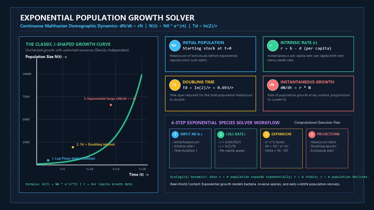
Definition: Calculate projected species population size N(t), intrinsic Malthusian growth rate r, population doubling time (Td), and instantaneous growth velocity dN/dt under density-independent conditions.
Governing Math Formula: Malthusian Exponential Growth: N(t) = N₀ · e^(r·t). Instantaneous Rate: dN/dt = r · N. Doubling Time: Td = ln(2) / r ≈ 0.69315 / r. Net Increase: ΔN = N(t) - N₀.
Target Applications: Provides real-time quantitative solutions in Biology for students, engineers, researchers, and finance professionals.
Exponential Species Population Growth Solver: Ecological Dynamics & Malthusian Modeling Guide
1. Introduction
In 1859, an Australian settler named Thomas Austin released just 24 European wild rabbits (Oryctolagus cuniculus) onto his estate in Victoria for weekend sport hunting. By the 1920s—a mere six decades later—Australia's rabbit population had exploded into an unfathomable 10 billion individuals, devouring millions of square kilometers of vegetation and triggering one of the most catastrophic ecological crises in modern history.
How can a handful of organisms multiply into billions in the blink of an evolutionary eye? Why do bacterial infections overpower host immune systems in a matter of hours? What mathematical rule governs the early colonizing surge of invasive plants, virus epidemics, and recovering wildlife populations?
The answer lies in Exponential Population Growth—the fundamental demographic process wherein a population's per-capita growth rate remains constant regardless of population size, causing total numbers to accelerate at a rate proportional to the population itself.
flowchart LR
    N0["Initial Stock N₀
(e.g., 24 Rabbits)"] -->|"Intrinsic Rate r > 0
(Births > Deaths)"| RATE["Per-Capita Speed r
dN/dt = r · N"]
    RATE -->|"Time t Elapsed"| EXP["Exponential Engine
N(t) = N₀ · e^(rt)"]
    EXP --> SURGE["Exponential Surge N(t)
J-Shaped Population Boom"]
    SURGE --> DOUBLING["Doubling Cycle Td
Td = ln(2) / r"]
Whether you are an ecology student analyzing wildlife management data, a microbiologist calculating bacterial doubling intervals in a fermenter, or an epidemiologist evaluating initial epidemic reproduction kinetics, understanding exponential growth is essential.
In this comprehensive guide, you will master the mathematical derivations, biological mechanisms, real-world case studies, and practical applications of the exponential growth model.
2. Definitions
2.1 Simple Everyday Definition
Exponential population growth occurs when a living population increases by a fixed percentage over regular intervals of time. Instead of adding a fixed number of new individuals each year (linear growth), the number of newborn offspring gets larger and larger in every successive generation because each new generation produces its own offspring.
2.2 Formal Technical Definition
In theoretical ecology and demography, continuous exponential growth is a density-independent demographic model described by the first-order ordinary differential equation:
Where:
- is the instantaneous rate of population change over time.
- is the total population size at time .
- is the instantaneous per-capita rate of increase (also known as the Malthusian parameter), defined as the per-capita birth rate () minus the per-capita death rate ().
When integrated with respect to time from an initial population at , it yields the continuous exponential function:
2.3 Vivid Real-World Analogies
The Compound Interest Analogy:
Imagine a bank account where your interest is not just paid out annually, but added to your principal balance every single microsecond. As your balance swells, the interest earned each second swells too. In population biology, every newborn organism represents new "capital" that immediately begins earning biological "interest" by reproducing.
The Snowball on a Mountain Peak:
A tiny snowball rolled down a snowy slope begins small and picks up only a few flakes. But as its surface area expands, every single rotation gathers exponentially more snow than the previous rotation. By the time it reaches the valley floor, it has transformed into an unstoppable avalanche.
3. History & Scientific Milestones
The mathematical modeling of expanding populations represents one of the earliest intersections between pure mathematics and empirical biology.
timeline
    title Milestones in Population Dynamics Modeling
    1760 : Leonhard Euler : Formulates earliest demographic age-structured population equations
    1798 : Thomas Robert Malthus : Publishes 'An Essay on the Principle of Population'
    1838 : Pierre François Verhulst : Introduces Logistic Equation to bound Malthusian growth
    1925 : Alfred J. Lotka : Establishes mathematical biophysics and intrinsic rate r
    1934 : Georgii Gause : Demonstrates exponential-to-logistic transitions in Paramecium
1970s : Conservation Biology : Integrates r-selection and minimum viable population dynamics- Leonhard Euler (1760): The renowned Swiss mathematician developed the first rigorous mathematical treatment of human mortality tables and stable age distributions, demonstrating how fertility schedules produce continuous exponential population trends.
- Thomas Robert Malthus (1798): In his landmark work An Essay on the Principle of Population, Malthus argued that while human agricultural production increases arithmetically ($1, 2, 3, 4, 5\dots$), unchecked biological populations grow geometrically ($1, 2, 4, 8, 16\dots$). This fundamental asymmetry directly inspired Charles Darwin and Alfred Russel Wallace in formulating the theory of natural selection.
- Pierre-François Verhulst (1838): Recognizing that real ecosystems possess limited carrying capacities (), Belgian mathematician Verhulst modified Malthus's exponential equation to create the celebrated logistic growth model.
- Alfred J. Lotka (1925) & Vito Volterra (1926): Formally established mathematical ecology, linking per-capita vital rates (), predator-prey oscillations, and competitive exclusion principles.
4. Core Concepts & Theoretical Principles
graph TD
    subgraph Core_Parameters["Foundational Demographic Parameters"]
        N0["Initial Size (N₀)"]
        r["Intrinsic Growth Rate (r = b - d)"]
        lambda["Finite Growth Multiplier (λ = e^r)"]
        Td["Doubling Time (Td = ln(2)/r)"]
    end

    subgraph Dynamics["Growth Regimes"]
        R_POS["r > 0 (λ > 1)
Exponential Expansion"]
        R_ZERO["r = 0 (λ = 1)
Stationary Population"]
        R_NEG["r < 0 (λ < 1)
Exponential Decline"]
    end

    r --> R_POS
    r --> R_ZERO
    r --> R_NEG
4.1 Intrinsic Rate of Increase ()
The intrinsic rate of increase (), measured in units of (, ), reflects the biotic potential of a species in an ideal, non-limiting environment:
Where , , , and per capita.
- When , births exceed deaths; the population undergoes exponential expansion.
- When , births exactly equal deaths; the population is in stationary equilibrium.
- When , deaths exceed births; the population suffers exponential decay toward extinction.
4.2 Finite Rate of Increase ()
In discrete time models (such as annual breeding seasons in deer or birds), biologists use the finite multiplication rate (lambda):
If a swan population increases by 15% in one year, , and its instantaneous rate is .
4.3 Doubling Time ()
The doubling time is the exact duration required for a population to double its initial size. Because the percentage growth rate is constant, the time required to grow from is identical to the time required to grow from .
4.4 The Two Phases of the J-Curve
- The Lag Phase: At small initial numbers (), absolute increases ($\Delta N$) appear slow and deceptive, even though the percentage rate is rapid.
- The Log/Acceleration Phase: Once becomes substantial, the product explodes, producing a nearly vertical upward trajectory on arithmetic graph axes.
5. Mathematical Formulas & Complete Derivations
5.1 Continuous Growth Equation Derivation
The rate of population change is directly proportional to current population size :
To solve this differential equation, we separate variables:
Integrate both sides from time (where ) to time (where ):
Exponentiate both sides with Euler's base :
5.2 Doubling Time () Derivation
To find the time when the population reaches double its starting size ():
Divide both sides by :
Take the natural logarithm ($\ln$) of both sides:
Rule of 70 in Ecology: For quick mental estimates, if a population grows at an annual percentage rate , its doubling time in years is approximately .
5.3 Complete Variable Breakdown
| Variable | Mathematical Symbol | Standard Units | Biological Meaning | Practical Interpretation |
|---|---|---|---|---|
| Initial Population | Individuals () | Starting stock size at | Founding flock, inoculum, or initial herd size | |
| Projected Population | $N(t)$ | Individuals () | Total headcount after elapsed time | Size of the population after growth cycle |
| Intrinsic Growth Rate | () | Instantaneous per-capita growth speed | Biological reproductive velocity ($b - d$) | |
| Time Elapsed | Years, Days, Hours | Total time span of observation | Duration of uninterrupted proliferation | |
| Doubling Time | Years, Days, Hours | Time span to double total numbers | Speed metric; smaller means faster growth | |
| Discrete Multiplier | Unitless ratio () | Step-wise annual growth multiplier | change; growth | |
| Instantaneous Velocity | Slope of growth curve at instant | Number of new individuals added per unit time |
6. Step-by-Step Computational Walkthrough
Let us calculate the demographic projection for an invasive carp population introduced into a lake:
flowchart TD
    S1["Step 1: Identify Known Parameters
N₀ = 80 fish, r = 0.35 yr⁻¹, t = 6 years"] --> S2["Step 2: Calculate Exponent Term
r · t = 0.35 × 6 = 2.10"]
    S2 --> S3["Step 3: Evaluate Natural Exponential e^(rt)
e^(2.10) ≈ 8.16617"]
    S3 --> S4["Step 4: Compute Final Size N(t)
N(6) = 80 × 8.16617 = 653 fish"]
    S4 --> S5["Step 5: Compute Doubling Time Td
Td = ln(2) / 0.35 = 0.69315 / 0.35 ≈ 1.98 years"]- Given:- Initial population- Per-capita annual growth rate (35% instantaneous growth)- Time horizon
- Compute the Growth Factor:
- Multiply by Initial Size:
- Determine Doubling Interval:(The fish population doubles roughly every 24 months!)
7. Visual Explanations & Model Selection Decision Trees
graph TD
    START{"What Ecological Conditions Apply?"}
    START -->|"Abundant Resources
Low Density
Early Colonization"| EXP_MODEL["Use Exponential Growth Model
dN/dt = rN
N(t) = N₀ · e^(rt)"]
    START -->|"Limited Space/Food
Density-Dependent Resistance
Long-Term Stability"| LOG_MODEL["Use Logistic Growth Model
dN/dt = rN · (1 - N/K)
Carrying Capacity K"]
    START -->|"Discrete Annual Seasons
Non-Overlapping Cohorts"| DISC_MODEL["Use Geometric Discrete Model
Nt = N₀ · λ^t
λ = e^r"]

    EXP_MODEL --> EX_EXP["Examples: Bacterial cultures in log phase, early viral transmission, invasive species vanguard"]
    LOG_MODEL --> EX_LOG["Examples: Forest deer herd, fish in closed pond, climax forest canopy trees"]
    DISC_MODEL --> EX_DISC["Examples: Annual flowering plants, migratory birds, univoltine insects"]
8. Comparative Analysis & Species Growth Benchmarks
8.1 Exponential vs. Logistic Growth Comparison
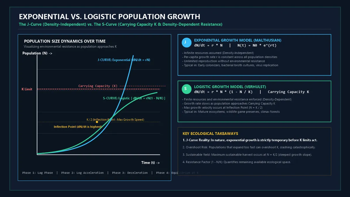
| Feature | Exponential Model (-Curve) | Logistic Model (-Curve) |
|---|---|---|
| Mathematical Equation | ||
| Environmental Limitation | Infinite resources assumed () | Resource limitation enforced () |
| Per-Capita Growth Rate | Constant () | Declines linearly as |
| Curve Geometry | Unbounded J-shaped curve | Sigmoidal S-shaped curve with asymptote |
| Density Dependence | Strictly density-independent | Strictly density-dependent |
| Typical Biological Context | Pioneer species, lab culture log phase, pests | Established climax communities, stable herds |
8.2 Intrinsic Rates & Doubling Times Across the Tree of Life
| Organism Class | Representative Species | Intrinsic Rate () | Typical Doubling Time () | Dominant Reproductive Strategy |
|---|---|---|---|---|
| Enteric Bacteria | Escherichia coli (in broth) | Binary fission (-selected) | ||
| Unicellular Fungus | Saccharomyces cerevisiae (Yeast) | Asymmetric cellular budding | ||
| Protozoan | Paramecium aurelia | Asexual cell division | ||
| Invasive Insect | Aedes aegypti (Mosquito) | High fecundity egg clutches | ||
| Small Rodent | Mus musculus (House Mouse) | Rapid polyestrous litters | ||
| Invasive Amphibian | Rhinella marina (Cane Toad) | 30,000 eggs per clutch | ||
| Large Ungulate | Cervus canadensis (Elk) | Single calf per maternal season | ||
| Apex Carnivore | Canis lupus (Gray Wolf) | Pack social breeding (-selected) | ||
| Modern Human | Homo sapiens (Global 1960s peak) | Long gestation, high parental care |
9. Practical Real-World Applications & Examples
Example 1: Bacterial Proliferation in Food Safety
A cutting board is contaminated with of Salmonella enterica. At warm ambient temperature (), the bacteria reproduce with an intrinsic rate ( or ). After : In just 6 hours, harmless contamination turns into an infectious, disease-causing threshold.
Example 2: Yeast Starter in Brewing Fermentation
A brewmaster pitches an initial culture of into a wort tank. The yeast expands at . To reach the desired pitching density of :
Example 3: Wildlife Reintroduction of Gray Wolves
In 1995, wildlife biologists released into Yellowstone National Park. With an abundance of elk prey and zero competitors, the population grew at . After :
Example 4: Algal Blooms in Agricultural Runoff Lakes
Excess phosphorus runoff triggers an exponential cyanobacterial bloom with initial density and . After : The lake turns turbid green, causing hypoxia and fish die-offs.
Example 5: Early Epidemic Viral Spread ( Kinetics)
In an immunologically naive population, a respiratory pathogen with generation interval and basic reproduction number has an early exponential rate . If initially : After :
10. In-Depth Case Studies
Case Study 1: The Reindeer of St. Matthew Island (1944–1966)
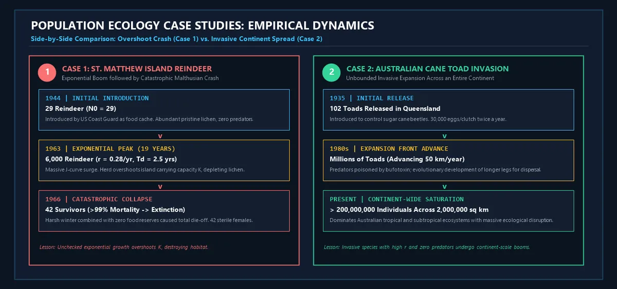
- Background: In 1944, the U.S. Coast Guard introduced 29 reindeer (Rangifer tarandus) to remote St. Matthew Island in the Bering Sea as a backup food cache.
- The Exponential Phase: The island had no wolves, no hunters, and pristine carpeted mats of lichen. The herd experienced near-maximal biotic potential (), doubling every 2.5 years. By 1963, the population had skyrocketed from .
- The Catastrophic Crash: Overgrazing decimated the island's slow-growing lichen reserves. During the harsh blizzard winter of 1963–1964, the herd underwent a catastrophic Malthusian die-off: over 99% of the reindeer starved, leaving just 42 living females and zero males, driving the herd to complete extinction.
- Key Takeaway: Unchecked exponential growth inevitably overshoots ecological carrying capacity, leading to severe resource destruction and population collapse.
Case Study 2: The Cane Toad Invasion of Australia (1935–Present)
- Background: In June 1935, 102 cane toads were released in northern Queensland sugar cane fields to control destructive beetles.
- Demographic Dynamics: Female cane toads lay up to twice a year. Native Australian predators (quolls, snakes, monitor lizards) had no evolutionary immunity to bufotoxin and died rapidly upon ingestion.
- Current Status: Free from predation, the cane toad population expanded across over at rates exceeding , with numbers surpassing 200 million individuals.
11. Advantages of the Exponential Model
- Analytical Simplicity: Requires only two primary input parameters ( and ), allowing rapid calculation without complex multi-variable computational models.
- High Accuracy During Early Phases: Provides an exact representation of initial colonization dynamics, microbial growth phases, and disease outbreak trajectories before density-dependent constraints occur.
- Foundation for Advanced Ecological Modeling: Serves as the mathematical baseline from which logistic models, Lotka-Volterra equations, and age-structured Leslie matrices are built.
- Standardized Doubling Metric: The doubling time provides a clear, universally understood metric for comparing growth velocities across widely diverse species.
12. Biological Limitations & Environmental Realities
While the exponential model is mathematically elegant, no biological population can grow exponentially forever. In nature, exponential growth is strictly temporary because:
- Resource Exhaustion: Rapidly expanding populations deplete essential nutrients, freshwater, breeding territories, and energy reserves.
- Accumulation of Toxic Byproducts: Microbial populations generate inhibitory metabolic wastes (e.g., ethanol in yeast fermentation, lactic acid in bacteria) that lower pH and halt replication.
- Density-Dependent Predation & Disease: Crowded populations suffer from increased pathogen transmission rates, heightened parasite loads, and enhanced predator attraction.
- Behavioral & Stress Feedback: Social mammals experience elevated glucocorticoid stress hormones, aggressive competition, and reduced maternal care at elevated densities.
13. Common Mistakes to Avoid
1. Mixing Up Time Units:
Always verify that your growth rate and time period use the same unit of time. If , you cannot plug in without converting years to days ().
2. Confusing (Continuous) with (Discrete):
Remember that , not $1 + r$. While for very small values of , they diverge significantly when growth rates are large.
3. Assuming $N(t)$ Represents an Unbroken Upper Limit:
Real populations fluctuate around trajectories due to environmental stochasticity, seasonal winter mortality, and resource cycles.
12. Frequently Asked Questions (FAQ)
What is the difference between geometric growth and exponential growth?
Geometric growth applies to organisms that reproduce in discrete, non-overlapping pulses or seasonal breeding cycles (e.g., annual flowers, deer mating in autumn), modeled as . Exponential growth applies to organisms with continuous, overlapping reproduction (e.g., bacteria, humans), modeled as .
Why is Euler's number () used in population growth?
Euler's number is the unique mathematical constant that arises naturally when compound growth occurs continuously at every infinitesimal instant of time.
How do you convert between doubling time () and intrinsic growth rate ()?
Use the exact identities:
What does a negative intrinsic growth rate () indicate?
A negative growth rate () indicates that per-capita mortality exceeds natality (). The population undergoes exponential decay, halving at intervals of , and will head toward extinction unless conditions improve.
What is the difference between -selected and -selected species?
- -selected species (e.g., bacteria, weeds, insects) prioritize high reproductive rates (), produce large numbers of offspring, invest little parental care, and thrive in unstable, open environments.
- -selected species (e.g., elephants, whales, humans) prioritize competitive ability, produce few offspring, invest heavily in parental care, and maintain populations near carrying capacity ().
Can a population with a low initial size () grow rapidly?
Yes. Although absolute increments ($\Delta N$) are small during the initial lag phase, the percentage growth rate is identical. Once the population surpasses a threshold size, total headcount surges dramatically.
How does immigration affect the exponential equation?
If net immigration occurs at a constant per-capita rate , the intrinsic rate simply becomes .
Why does the exponential growth curve look straight on a logarithmic graph?
Taking the natural logarithm of both sides of yields the linear equation , where is the constant linear slope and is the y-intercept.
When does exponential growth transition into logistic growth?
As population size approaches environmental carrying capacity (), density-dependent factors reduce birth rates and increase death rates, causing the slope to decelerate toward zero at .
What is the Rule of 70?
The Rule of 70 is a mental shortcut to calculate doubling time: divide by the percentage growth rate (e.g., at 7% annual growth, doubling time is ).
15. Expert Tips & Best Practices in Ecological Modeling
- Plot on Semi-Logarithmic Axes: Always plot population data on a semi-log scale ($\ln(N)$ vs. ). A true exponential phase will form a straight line, making deviations from equilibrium immediately noticeable.
- Cross-Check Environmental Carrying Capacities (): Never extrapolate exponential models beyond short-term horizons without evaluating the host ecosystem's food and territorial limits.
- Account for Age Structure: If a population contains disproportionately post-reproductive or juvenile cohorts, observed growth will lag behind theoretical intrinsic rate until a stable age distribution is reached.
- Incorporate Stochastic Buffers in Conservation: For endangered species with , random demographic fluctuations (e.g., bad weather, sex-ratio skews) can cause extinction even if .
16. Summary Checklist
- ✔ Initial Stock (): Set the baseline population count at .
- ✔ Intrinsic Rate (): Determine instantaneous per-capita growth speed ($b - d$).
- ✔ Time Horizon (): Ensure matching units between and (days, months, years).
- ✔ Evaluate Doubling Period (): Compute for intuitive growth assessment.
- ✔ Calculate Projected Size ($N(t)$): Execute .
- ✔ Assess Ecological Context: Confirm whether density-independent assumptions remain valid.
Additional Technical Guidelines & Measurement Standards
When conducting calculations for Exponential Species Population Growth Solver, maintaining quantitative precision and verifying input parameter boundaries is essential for reliable scenario evaluation. Always verify that raw numerical inputs are measured using standardized instrumentation, and double-check unit conversions prior to applying outputs in commercial, industrial, or academic projects.
For quantitative unit conversions and scientific calculations, always maintain at least four decimal places of precision during intermediate arithmetic stages before rounding final results. When preparing technical reports, laboratory documentation, or financial forecasts, cross-verify all output variables against established international measurement standards (such as SI, NIST, and ISO metric benchmarks) to guarantee consistent analytical rigor across all computational workflows.
MathsLover.com delivers this interactive solver 100% free of charge to foster global mathematical literacy, educational accessibility, and data-driven problem solving across scientific, technical, and academic communities worldwide.