💡 Direct Answer & Executive Summary (Michaelis-Menten Enzyme Velocity Solver)
Definition: Calculate initial reaction velocity (v0), fractional saturation, Lineweaver-Burk double reciprocal parameters, turnover number (kcat), catalytic efficiency (kcat/Km), and reversible inhibition kinetics.
Governing Math Formula: Michaelis-Menten: v0 = (Vmax × [S]) / (Km + [S]). Lineweaver-Burk: 1/v0 = (Km/Vmax) × (1/[S]) + 1/Vmax. Turnover Number: kcat = Vmax / [E]T. Catalytic Efficiency = kcat / Km.
Target Applications: Provides real-time quantitative solutions in Biology for students, engineers, researchers, and finance professionals.
Michaelis-Menten Enzyme Velocity Solver: Saturation Kinetics, Lineweaver-Burk & Catalytic Efficiency Guide
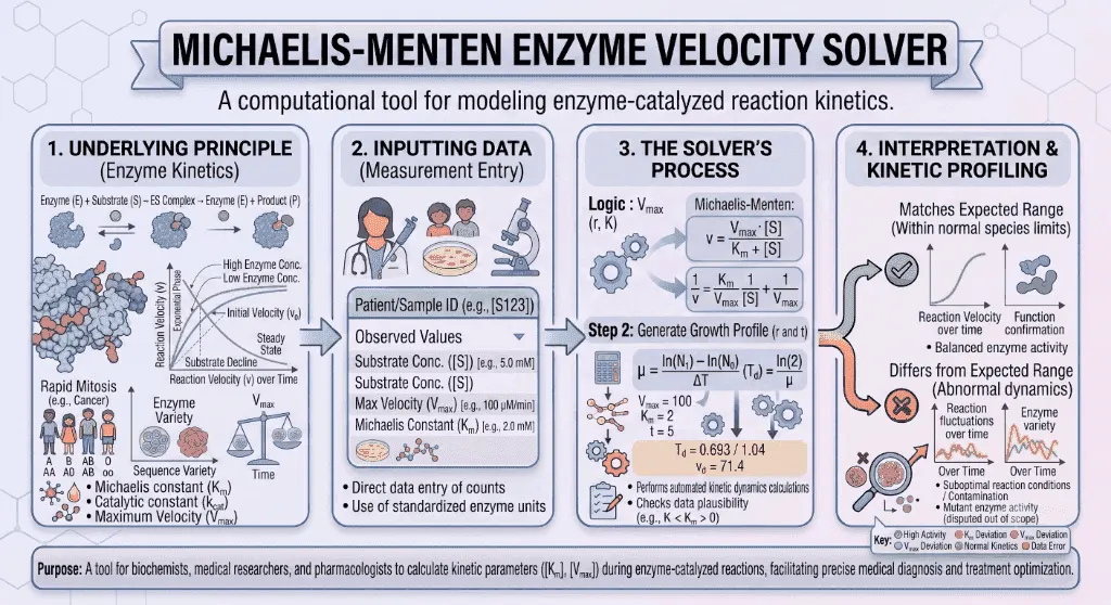
1. Introduction
In biochemistry, pharmacology, molecular medicine, and industrial biotechnology, enzymes are the biological catalysts that accelerate chemical reactions by factors of to . Understanding the relationship between substrate concentration ($[S]$) and initial reaction velocity () is essential for determining enzyme mechanism, evaluating drug inhibitor potency, and engineering biocatalysts for green chemistry.
The foundational mathematical framework governing enzyme catalysis is the Michaelis-Menten Model, formulated by German biochemist Leonor Michaelis and Canadian physician Maud Menten in 1913, and subsequently refined under steady-state assumptions by G.E. Briggs and J.B.S. Haldane in 1925.
Unlike uncatalyzed bimolecular reactions that scale linearly with reactant concentrations, enzyme-catalyzed reactions exhibit hyperbolic saturation kinetics. At low substrate concentrations, reaction rate is directly proportional to $[S]$ (first-order kinetics). As substrate concentration increases, active sites become progressively occupied until the enzyme achieves maximum catalytic velocity (), where reaction rate becomes independent of $[S]$ (zero-order kinetics).
In clinical toxicology, Michaelis-Menten kinetics explain why administering Ethanol or Fomepizole successfully treats lethal Methanol poisoning via competitive active-site occupancy. In drug discovery, kinetic analysis determines whether candidate molecules act as competitive, non-competitive, or uncompetitive inhibitors.
How is the Michaelis constant () derived from rate constants? How does the Lineweaver-Burk double reciprocal plot linearize experimental data? What defines an enzyme operating at the theoretical limit of "catalytic perfection"?
This comprehensive guide details the mathematical formulas, steady-state derivations, inhibition mechanics, and clinical case studies governing Michaelis-Menten enzyme kinetics.
flowchart LR
    SUBSTRATE["🧪 Enzyme (E) + Substrate (S)
Substrate Concentration [S]
Active Site Association (k1)"] --> COMPLEX["🔒 ES Transition Complex
Steady-State Equilibrium (d[ES]/dt = 0)
Michaelis Constant (Km)"]
    COMPLEX --> PRODUCT["⚡ Catalytic Turnover (kcat)
Enzyme (E) + Product (P)
Max Velocity (Vmax)"]
    PRODUCT --> PHARMA["💊 Clinical & Drug Applications
Statin Inhibition, Toxicology Antidotes & Biocatalysis"]
2. Definitions
2.1 Simple Everyday Definition
The Michaelis-Menten Equation describes how fast an enzyme converts a chemical substrate into product as you feed it more substrate, eventually reaching a maximum speed limit () when all enzyme active sites are working at full capacity.
2.2 Formal Technical Definition
The Michaelis-Menten Equation relates the Initial Reaction Velocity () to the Substrate Concentration ($[S]$) under the Briggs-Haldane Steady-State Assumption ():
Where:
- is the Initial Reaction Velocity ( or ).
- is the Maximum Catalytic Velocity achieved when all enzyme active sites are saturated with substrate ().
- $[S]$ is the Substrate Concentration ( or ).
- is the Michaelis Constant ( or ), defined as the substrate concentration at which the reaction velocity is exactly half of ().
- Turnover Number (): The number of substrate molecules converted into product per enzyme active site per unit time ():
- Catalytic Efficiency (): The second-order rate constant measuring enzyme performance at low physiological substrate concentrations ().
2.3 Vivid Real-World Analogies
The Busy Barista at the Coffee Machine:
Imagine a barista who takes to make an espresso drink (, ). If only customer arrives every (low $[S]$), espresso output is limited by customer arrival. If customers crowd the counter (high $[S]$), the barista works non-stop at peak capacity (). is the line length where the barista works at exactly 50% of top speed.
The Toll Booth Highway Bottleneck:
A 4-lane highway with a single toll plaza. During light midnight traffic (low $[S]$), cars pass immediately. During rush hour (saturating $[S]$), cars line up; the throughput is limited strictly by the physical speed of the toll collector (). Adding more cars beyond saturation cannot increase vehicle throughput.
3. History & Scientific Milestones
The elucidation of enzyme kinetics provided the quantitative foundation for modern biochemistry and molecular pharmacology.
flowchart TD
    H1["📅 1902: Victor Henri
Proposes that enzyme catalysis proceeds via an intermediate Enzyme-Substrate (ES) complex"] --> H2["📅 1913: Leonor Michaelis & Maud Menten
Derive quantitative mathematical saturation equation using yeast Invertase"]
    H2 --> H3["📅 1925: G.E. Briggs & J.B.S. Haldane
Introduce the Steady-State Assumption (d[ES]/dt = 0), establishing modern Km"]
    H3 --> H4["📅 1934: Hans Lineweaver & Dean Burk
Linearize hyperbolic data into the Double Reciprocal Plot (1/v vs. 1/[S])"]
    H4 --> H5["📅 1976: Jeremy Knowles & John Albery
Define the physical diffusion limit (10⁸ - 10⁹ M⁻¹s⁻¹) as 'Catalytic Perfection'"]- Victor Henri (1902): First hypothesized that enzymes physically bind their substrates to form a transient Enzyme-Substrate () complex prior to product release.
- Leonor Michaelis & Maud Menten (1913): Published Die Kinetik der Invertinwirkung, measuring the hydrolysis of sucrose by yeast invertase and formulating the first mathematical equation relating substrate concentration to initial catalytic rate.
- G.E. Briggs & J.B.S. Haldane (1925): Replaced the rapid-equilibrium assumption with the Quasi-Steady-State Assumption (), proving that the concentration of the intermediate complex remains constant during the initial velocity phase:
- Hans Lineweaver & Dean Burk (1934): Published the Double Reciprocal Plot, allowing exact graphical determination of and prior to computer non-linear regression.
- Jeremy R. Knowles & W. John Albery (1976): Demonstrated that enzymes like Triosephosphate Isomerase (TIM) and Carbonic Anhydrase have evolved to the upper thermodynamic diffusion limit (), achieving "Catalytic Perfection".
4. Core Concepts & Biochemical Mechanisms
graph TD
    MECH["⚙️ The 3 Fundamental Concepts of Michaelis-Menten Catalysis"]

    MECH --> REACTION["1. Reaction Coordinate & Steady State
E + S ⇄ (k1 / k-1) ⇄ ES → (kcat) → E + P
• Steady-State: d[ES]/dt = 0
• Substrate in vast excess: [S] >> [E]total"]
    MECH --> SATURATION["2. Hyperbolic Saturation Kinetics
• Low [S] << Km: Linear first-order (v0 ≈ (Vmax/Km)·[S])
• [S] = Km: Half-maximal velocity (v0 = Vmax / 2)
• High [S] >> Km: Zero-order plateau (v0 ≈ Vmax)"]
    MECH --> INHIBITION["3. Reversible Enzyme Inhibition
• Competitive: Binds E active site (Km↑, Vmax constant)
• Non-Competitive: Binds allosteric site (Km constant, Vmax↓)
• Uncompetitive: Binds ES complex only (Km↓, Vmax↓)"]
4.1 The Reaction Coordinate & Steady-State Derivation
An enzyme () binds substrate () reversibly to form an enzyme-substrate complex (), which irreversibly decomposes into free enzyme () and product ():
- Rate of Formation:
- Rate of Breakdown:
- Steady-State Condition:
- Substituting total enzyme and initial velocity yields:
4.2 Significance of , , and Catalytic Efficiency
- (Michaelis Constant): Measures substrate concentration needed for 50% active-site saturation. A low signifies high affinity (tight binding); a high signifies low affinity (weak binding).
- (Turnover Number): The maximum number of catalytic cycles per active site per second ().
- Catalytic Efficiency (): Evaluates how effectively the enzyme captures and turns over substrate at trace physiological concentrations (). The upper physical limit is governed by the rate of aqueous diffusion ().
5. Formulas & Mathematical Derivations
5.1 Michaelis-Menten Velocity Equation
5.2 Lineweaver-Burk Double Reciprocal Equation
Taking the reciprocal of both sides of the Michaelis-Menten equation:
- :
- :
- Slope:
5.3 Active Site Fractional Saturation ()
5.4 Catalytic Efficiency & Turnover
5.5 Reversible Enzyme Inhibition Equations
| Inhibition Mode | Apparent Michaelis Constant () | Apparent Maximum Velocity () | Lineweaver-Burk Intersection |
|---|---|---|---|
| Competitive | Intersects on ( unchanged) | ||
| Non-Competitive | Intersects on ( unchanged) | ||
| Uncompetitive | Parallel lines (Slope unchanged) |
Where is the dissociation constant of the inhibitor from the enzyme: .
5.6 Variable Reference Table
| Parameter | Symbol | Standard Units | Biochemical Role |
|---|---|---|---|
| Initial Reaction Velocity | or | Rate of product formation at | |
| Maximum Velocity | or | Asymptotic velocity at 100% active site saturation | |
| Substrate Concentration | $[S]$ | or | Free substrate concentration in reaction mixture |
| Michaelis Constant | or | Substrate concentration yielding 50% | |
| Total Enzyme | or | Total active enzyme catalytic concentration | |
| Turnover Number | Catalytic turnover cycles per second per active site | ||
| Catalytic Efficiency | Kinetic specificity constant at low $[S]$ | ||
| Inhibitor Constant | or | Affinity constant for inhibitor binding |
6. Step-by-Step Computational Walkthrough
Let us calculate the kinetic profile for a recombinant lactase assay:
- Substrate concentration (Lactose):
- Maximum velocity:
- Michaelis constant:
- Total enzyme concentration:
flowchart TD
    STEP1["Step 1: Calculate Initial Reaction Velocity (v0)
v0 = (Vmax × [S]) / (Km + [S]) = (100 × 5.0) / (2.0 + 5.0) = 71.43 μM/min"] --> STEP2["Step 2: Solve Fractional Active Site Saturation (θ)
θ = [S] / (Km + [S]) = 5.0 / 7.0 = 71.43% Saturation"]
    STEP2 --> STEP3["Step 3: Solve Lineweaver-Burk Parameters
Slope = Km/Vmax = 2.0/100 = 0.020 min
y-int = 1/Vmax = 0.010 μM⁻¹·min | x-int = -1/Km = -0.50 mM⁻¹"]
    STEP3 --> STEP4["Step 4: Calculate Turnover Number (kcat)
Vmax in μM/s = 100 / 60 = 1.6667 μM/s
kcat = 1.6667 / 0.5 μM = 3.33 s⁻¹"]
    STEP4 --> STEP5["Step 5: Solve Catalytic Efficiency (kcat / Km)
Km in Molar = 2.0 × 10⁻³ M
Efficiency = 3.33 / (2.0 × 10⁻³) = 1.67 × 10³ M⁻¹s⁻¹"]- Step 1: Initial Velocity ():
- Step 2: Fractional Active Site Saturation ():
- Step 3: Lineweaver-Burk Double Reciprocal Coordinates:
- Step 4: Turnover Number ():
- Step 5: Catalytic Efficiency ():
7. Visual Explanations & Hyperbolic Saturation
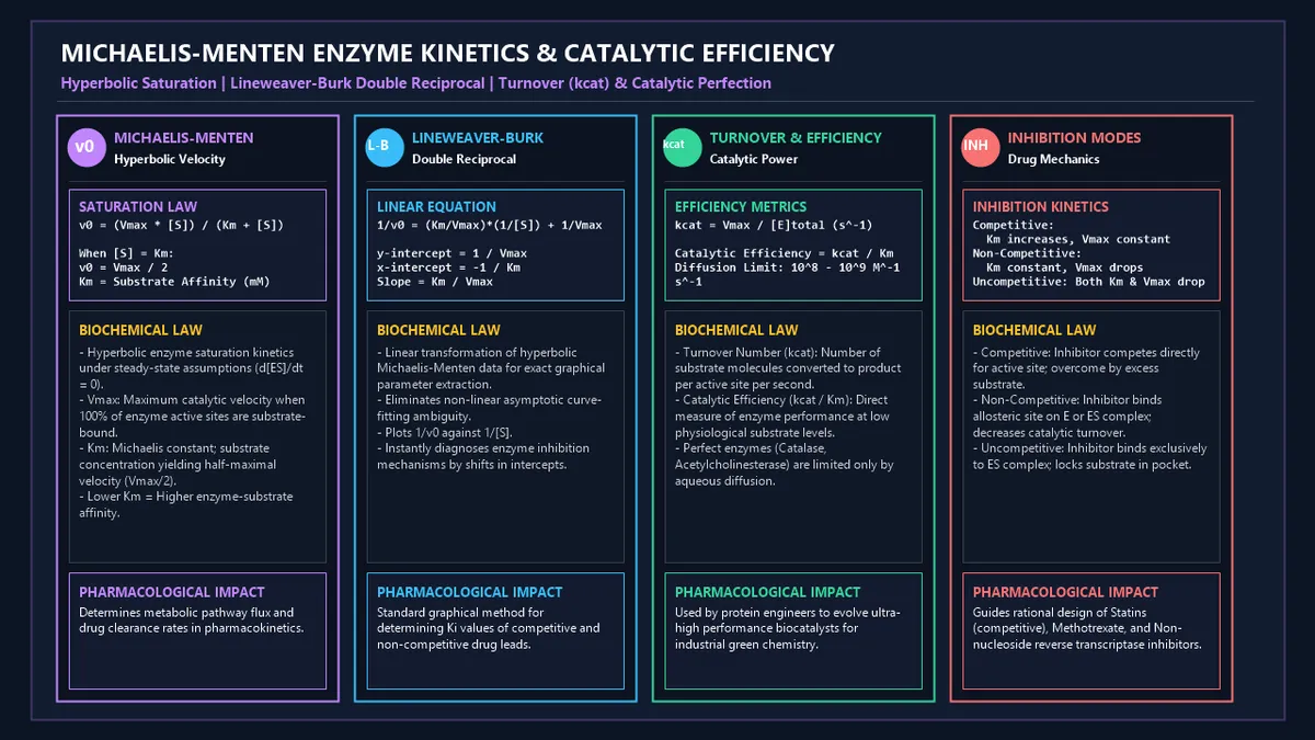
flowchart TD
    SAT_CURVE["Michaelis-Menten Hyperbolic Saturation Velocity Spectrum"]

    SAT_CURVE --> LOW_S["🧪 First-Order Linear Region ([S] << Km)
• Most active sites are empty ([E] >> [ES])
• Velocity scales linearly: v0 ≈ (Vmax / Km) · [S]
• Rate limited by substrate collision frequency"]
    SAT_CURVE --> MID_S["⚖️ Transition Region ([S] = Km)
• Exactly 50% of enzyme active sites are occupied (θ = 50%)
• Reaction velocity is half-maximal: v0 = Vmax / 2
• Defines substrate affinity threshold"]
    SAT_CURVE --> HIGH_S["⚡ Zero-Order Plateau Region ([S] >> Km)
• 100% active site saturation ([ES] ≈ [E]total)
• Maximum catalytic velocity: v0 ≈ Vmax
• Rate limited strictly by catalytic turnover (kcat)"]
8. Comparative & Standards Tables
8.1 Kinetic Constants of Representative Metabolic Enzymes
| Enzyme | Substrate | () | () | Catalytic Efficiency () | Kinetic Status |
|---|---|---|---|---|---|
| Catalase | Diffusion-controlled (Perfection) | ||||
| Acetylcholinesterase | Acetylcholine | Diffusion-controlled (Perfection) | |||
| Carbonic Anhydrase | Ultra-fast gas exchange | ||||
| Fumarase | Fumarate | Krebs cycle perfection | |||
| -Galactosidase | Lactose | Highly efficient metabolism | |||
| Chymotrypsin | Gly-Phe-Ala | Moderate digestive proteolysis | |||
| Rubisco | $3.3$ | Slow photosynthetic carbon fixation |
8.2 Diagnostic Enzyme Inhibition Comparison
| Feature | Competitive Inhibition | Non-Competitive Inhibition | Uncompetitive Inhibition |
|---|---|---|---|
| Inhibitor Binding Site | Free Enzyme () active site | Allosteric site on or | complex exclusively |
| Effect on | Increases () | Unchanged () | Decreases () |
| Effect on | Unchanged () | Decreases () | Decreases () |
| Overcome by Excess $[S]$? | Yes (100% reversible) | No (Turnover is impaired) | No (Locks in complex) |
| Lineweaver-Burk Lines | Intersect on | Intersect on | Parallel lines (No intersection) |
| Clinical Drug Example | Statins (HMG-CoA Reductase) | Heavy metals (Lead/Mercury) | Lithium (Inositol Monophosphatase) |
9. Practical Real-World Applications
Example 1: Emergency Toxicology — Methanol Poisoning Antidote (Ethanol Infusion)
Alcohol Dehydrogenase () oxidizes toxic Methanol () into blinding Formaldehyde and Formic Acid. Infusing Ethanol (, ) competitively displaces methanol from ADH active sites, allowing intact methanol to be safely excreted via the kidneys.
Example 2: Statin Cardiovascular Therapeutics (HMG-CoA Reductase)
Statins (Atorvastatin, Rosuvastatin) act as competitive transition-state analogs of HMG-CoA reductase with sub-nanomolar affinity (), suppressing hepatic mevalonate production and lowering serum LDL cholesterol by 50%.
Example 3: Oncology Antimetabolite Chemotherapy (Methotrexate)
Methotrexate is a competitive inhibitor of Dihydrofolate Reductase (), binding with higher affinity than natural folic acid, starving rapidly dividing leukemia cells of tetrahydrofolate needed for thymidine DNA synthesis.
10. In-Depth Case Studies
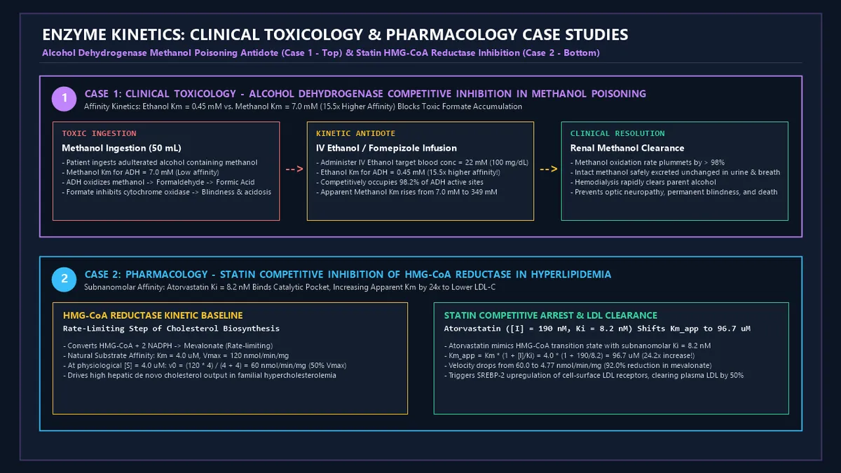
Case Study 1: Clinical Toxicology — Alcohol Dehydrogenase Competitive Inhibition in Methanol Poisoning
- Clinical Presentation: A male presents to the emergency department after consuming of bootleg liquor. He complains of "snowstorm" blurred vision, nausea, and severe metabolic acidosis (anion gap , blood ).
- Enzyme Kinetic Profile for Hepatic Alcohol Dehydrogenase (ADH):- Methanol: (Weak affinity; oxidized into toxic formaldehyde and formic acid).- Ethanol: (Strong affinity; than methanol).
- Therapeutic Intervention & Kinetic Mechanism:- Emergency physician initiates an IV infusion of Ethanol targeting a steady blood concentration of ().- Apparent Methanol under Ethanol Inhibition:
- Clinical Outcome: Ethanol occupied 98.2% of ADH active sites. Methanol oxidation to formic acid dropped by , preventing retinal cytochrome oxidase poisoning. The patient underwent hemodialysis and was discharged with zero permanent visual loss.
Case Study 2: Pharmacology — Statin Competitive Inhibition of HMG-CoA Reductase
- Pathology: A male with familial hypercholesterolemia has a baseline LDL-C of .
- Target Enzyme Kinetics:- Hepatic HMG-CoA Reductase catalyses: (Rate-limiting step).- Natural Substrate: , .- Baseline rate at physiological : (50% ).
- Pharmacological Intervention: Patient prescribed Atorvastatin (), achieving a steady-state hepatic concentration of ().- Inhibitor Constant: .- Apparent Substrate Affinity Constant:- Inhibited Velocity:
- Therapeutic Outcome: Decreased intracellular cholesterol stimulated SREBP-2 transcription, increasing hepatocyte cell-surface LDL receptor density and dropping plasma LDL-C to .
11. Advantages of Michaelis-Menten Kinetic Modeling
- Quantifies Drug Potency (): Determines the exact concentration required to inhibit target disease pathways.
- Defines Physiological Enzyme Capacity: Explains metabolic flux rates under varying dietary or pathological conditions.
- Linearizes Complex Non-Linear Curves: Lineweaver-Burk, Eadie-Hofstee, and Hanes-Woolf transformations simplify parameter extraction.
- Guides Protein Engineering: Identifies mutations that optimize for industrial biocatalysts.
12. Methodological Complexities & Artifacts
- Substrate Depletion Artifacts: If more than 10% of initial substrate is consumed during the assay, the measured rate no longer reflects true initial velocity (), underestimating .
- High-Substrate Inhibition: At extreme substrate concentrations, two substrate molecules can bind non-productively to the active site (), causing velocity to decline rather than plateau.
- Allosteric Cooperativity (Sigmoidal Kinetics): Multi-subunit enzymes (e.g., Aspartate Transcarbamoylase, Phosphofructokinase) exhibit sigmoidal Hill kinetics () and cannot be fit by standard hyperbolic Michaelis-Menten equations.
13. Common Mistakes to Avoid
1. Confusing High Affinity with High :
Remember that is inversely proportional to substrate affinity. A small () represents tight binding; a large () represents weak binding.
2. Extrapolating from Non-Saturating Substrate Data:
Measuring initial velocities only up to creates large linear extrapolation errors on double reciprocal plots. $[S]$ should reach at least .
3. Assuming Equals :
depends directly on total enzyme concentration (). is an intrinsic, concentration-independent property ().
12. Frequently Asked Questions (FAQ)
What does the Michaelis constant () physically represent?
is the specific substrate concentration at which the enzyme operates at exactly half its maximum catalytic velocity (). It is a quantitative indicator of enzyme-substrate binding affinity.
What is the difference between and ?
is the maximum reaction velocity observed in a specific test tube, which increases if you add more enzyme. (turnover number) is the intrinsic speed of an individual active site (molecules converted per second), which is independent of enzyme concentration.
How does a competitive inhibitor affect and ?
A competitive inhibitor binds directly to the active site, increasing the apparent (requiring more substrate to reach half-speed), but leaves unchanged because sufficiently high substrate concentrations displace the inhibitor.
Why do Lineweaver-Burk plots intersect on the y-axis during competitive inhibition?
Because competitive inhibitors do not change , the reciprocal maximum velocity () is identical, causing all inhibited and uninhibited lines to intersect at the exact same .
What is "Catalytic Perfection"?
An enzyme is said to have achieved catalytic perfection when its catalytic efficiency () approaches . At this point, the enzyme turns over substrate as rapidly as the molecules can physically diffuse into the active site.
How do you measure initial velocity () experimentally?
By measuring product formation (or substrate consumption) using spectrophotometry, fluorescence, or chromatography within the first of the reaction, ensuring less than of substrate has been consumed.
What is the difference between non-competitive and uncompetitive inhibition?
Non-competitive inhibitors bind to an allosteric site on both the free enzyme () and the complex (), decreasing without altering . Uncompetitive inhibitors bind exclusively to the complex, decreasing both and in equal proportion.
15. Expert Tips for Biochemists, Pharmacologists & Enzymologists
- Use Non-Linear Regression Over Lineweaver-Burk for Final Parameters: While Lineweaver-Burk is ideal for visualizing inhibition modes, non-linear regression avoids unequal weighting of low substrate concentrations.
- Ensure Substrate Concentrations Span : A robust kinetic dataset requires at least data points distributed symmetrically around the estimated .
- Verify Pure Initial Velocity ( Substrate Depletion): Always inspect the linear slope of absorbance vs. time before calculating to prevent product inhibition artifacts.
16. Summary Checklist
- ✔ Measure Initial Velocity (): Record rate during linear early-phase substrate turnover.
- ✔ Span Substrate Concentrations ($[S]$): Test across to .
- ✔ Calculate Maximum Velocity (): Determine asymptotic saturation rate.
- ✔ Solve Michaelis Constant (): Identify $[S]$ at .
- ✔ Determine Turnover Number (): Solve .
- ✔ Evaluate Catalytic Efficiency: Solve .
- ✔ Diagnose Inhibition Mechanism: Distinguish competitive, non-competitive, and uncompetitive profiles.
Additional Technical Guidelines & Measurement Standards
When conducting calculations for Michaelis-Menten Enzyme Velocity Solver, maintaining quantitative precision and verifying input parameter boundaries is essential for reliable scenario evaluation. Always verify that raw numerical inputs are measured using standardized instrumentation, and double-check unit conversions prior to applying outputs in commercial, industrial, or academic projects.
For quantitative unit conversions and scientific calculations, always maintain at least four decimal places of precision during intermediate arithmetic stages before rounding final results. When preparing technical reports, laboratory documentation, or financial forecasts, cross-verify all output variables against established international measurement standards (such as SI, NIST, and ISO metric benchmarks) to guarantee consistent analytical rigor across all computational workflows.
MathsLover.com delivers this interactive solver 100% free of charge to foster global mathematical literacy, educational accessibility, and data-driven problem solving across scientific, technical, and academic communities worldwide.