💡 Direct Answer & Executive Summary (Cell Doubling Time & Growth Rate Solver)
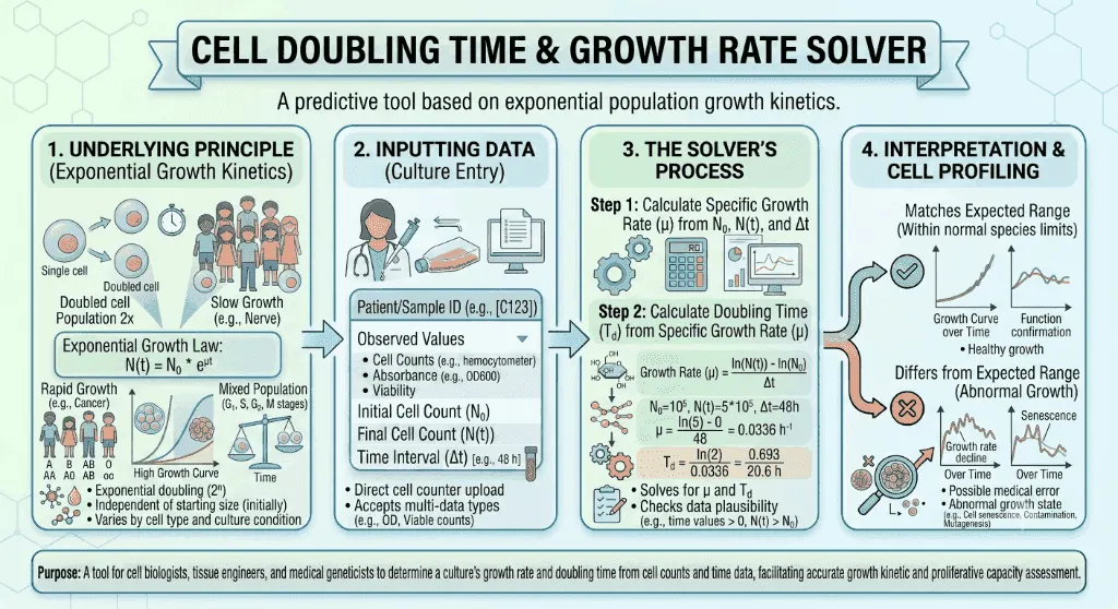
Definition: Calculate specific growth rate (μ), doubling time (Td), population doublings (PD), and fold-expansion from initial and final cell counts across time.
Governing Math Formula: Specific Growth Rate: μ = [ln(Nt) - ln(N0)] / Δt. Doubling Time: Td = ln(2) / μ = 0.69315 / μ. Population Doublings: PD = ln(Nt / N0) / ln(2) = 3.322 × log10(Nt / N0).
Target Applications: Provides real-time quantitative solutions in Biology for students, engineers, researchers, and finance professionals.
Cell Doubling Time & Growth Rate Solver: Culture Kinetics, Specific Growth Rate & Bioprocess Guide
1. Introduction
Cellular proliferation is the fundamental engine driving development, tissue regeneration, cancer progression, and industrial biotechnology. Whether expanding stem cells for regenerative medicine, producing monoclonal antibodies in biopharmaceutical reactors, or screening chemotherapeutic drugs against patient-derived tumor lines, mastering cell culture growth kinetics is critical for reproducibility, quality control, and process optimization.
The quantitative behavior of proliferating cells is governed by two foundational metrics: the Specific Growth Rate (), which measures instantaneous proliferation velocity, and the Doubling Time (), which defines the exact duration required for a cell population to double in number.
In biomanufacturing, shifts in doubling time indicate batch contamination, nutrient depletion, or cellular genetic drift. In oncology, rapid doubling times correlate directly with tumor aggressiveness, while prolonged doubling times confirm drug-induced cytostatic cell cycle arrest.
How are growth rate () and doubling time () derived mathematically from experimental counts? What biological mechanisms dictate the four in vitro culture phases? How do scientists distinguish between passage number and cumulative population doublings?
This comprehensive guide delivers the mathematical derivations, biophysical mechanisms, laboratory protocols, and bioprocess applications of cell doubling kinetics.
flowchart LR
    SEED["🧫 Initial Seeding
Count N₀ at Time t₀
(e.g., 1.0 × 10⁵ cells)"] --> HARVEST["🔬 Final Harvest
Count Nₜ at Time t
(e.g., 5.0 × 10⁵ cells at 48h)"]
    HARVEST --> SOLVER["🧮 Growth Kinetics Solver
Specific Growth Rate (μ)
Doubling Time (Td) & PDs"]
    SOLVER --> SCALE["🏭 Bioprocess & Clinical Action
Bioreactor Scaling, Passaging & Quality Control"]
2. Definitions
2.1 Simple Everyday Definition
Cell Doubling Time () is the amount of time it takes for a living population of cells to double in total count under continuous logarithmic growth. Specific Growth Rate () is the speed of cellular multiplication per unit of time.
2.2 Formal Technical Definition
The Specific Growth Rate () is the instantaneous rate of population increase per unit biomass or cell number, defined by the first-order differential equation of exponential growth:
Rearranging for the time interval :
The Doubling Time ( or ) is the exact period required for the population to double ():
2.3 Vivid Real-World Analogies
The Compound Interest Bank of Cells:
Imagine a bank account where your principal balance automatically compounds continuously. If you start with $100,000 and compound at an instantaneous rate $\mu = 0.0335\text{ per hour}$, your balance doubles every $20.7\text{ hours}$. Cells do not divide on a linear conveyor belt—each newly divided daughter cell immediately becomes an active factory for the next round of doubling ($2 \rightarrow 4 \rightarrow 8 \rightarrow 16 \rightarrow 2^n$).
The Factory Assembly Line Clock:
Think of the eukaryotic cell cycle as an automated four-station assembly line (). The Doubling Time represents the total time required for a product to complete the entire loop. If a checkpoint stalls (e.g., DNA damage in ), the assembly line clock slows, and the doubling time extends from to several days.
3. History & Scientific Milestones
The mathematical modeling of population kinetics transformed biology from descriptive taxonomy into an exact biophysical science.
flowchart TD
    M1["📅 1870s: Robert Koch & Louis Pasteur
Isolate pure bacterial cultures; establish exponential colony multiplication"] --> M2["📅 1942: Jacques Monod
Formulates Monod Equation linking substrate concentration to specific growth rate μ"]
    M2 --> M3["📅 1950s: Renato Dulbecco
Develops animal cell plaque assays and establishes in vitro mammalian kinetics"]
    M3 --> M4["📅 1961: Leonard Hayflick
Discovers finite replicative lifespan (~50 doublings) in human somatic fibroblasts"]
    M4 --> M5["📅 1980s: Industrial Biomanufacturing
Applies kinetic fed-batch modeling for recombinant monoclonal antibody CHO production"]- Robert Koch & Louis Pasteur (1870s): Developed solid agar culture media and broth fermentation, demonstrating that microorganisms multiply exponentially rather than generating spontaneously.
- Jacques Monod (1942): Published his landmark doctoral thesis on bacterial growth kinetics, deriving the Monod Equation relating specific growth rate () to limiting nutrient substrate concentration ():
- Renato Dulbecco (1950s): Pioneered quantitative animal virology and mammalian cell culture techniques, defining the kinetics of contact inhibition and monolayer saturation density.
- Leonard Hayflick (1961): Overturned Alexis Carrel's dogma of cellular immortality by proving that normal human primary somatic cells possess a finite replicative capacity of approximately (the Hayflick Limit), driven by telomere erosion.
- Modern Bioprocess Engineering (1980s–Present): Integrated real-time automated off-gas analysis and capacitance biomass sensors to dynamically monitor and in industrial bioreactors.
4. Core Concepts & Biophysical Mechanics
graph TD
    PHASE["🧫 The 4 In Vitro Culture Growth Phases"]

    PHASE --> LAG["1. Lag Phase (Adaptation)
• Cell attachment & spreading
• Enzyme induction & ribosome synthesis
• Zero net population increase (μ ≈ 0)"]
    PHASE --> LOG["2. Log / Exponential Phase (Optimal)
• Constant maximal growth rate (μ = μmax)
• Rapid binary division (2ⁿ)
• True Doubling Time (Td) measured here!"]
    PHASE --> STAT["3. Stationary Phase (Confluence)
• Contact inhibition & cell-cell contact
• Nutrient exhaustion & waste buildup (Lactate, NH₄⁺)
• Division rate equals death rate (μ = 0)"]
    PHASE --> DEATH["4. Death / Decline Phase
• Apoptotic caspase activation & lysis
• Viability drops below 70%
• Negative growth rate (μ < 0)"]
4.1 The Four Culture Growth Phases
- Lag Phase: Immediately following inoculation or passaging, cells recover from trypsinization stress, express adhesion integrins, and upregulate metabolic enzymes. No cell division occurs ().
- Log (Exponential) Phase: Cells enter active, uninhibited exponential growth where division occurs at a constant maximal specific growth rate (). This is the only phase where doubling time can be accurately calculated!
- Stationary Phase: As cells reach monolayer confluence, surface contact triggers contact inhibition via cadherin signaling. Nutrient levels drop, toxic metabolites (lactate and ammonia) accumulate, and proliferation balances cell death.
- Death Phase: Toxic waste and nutrient depletion activate programmed cell death (apoptosis) and membrane necrosis, causing total viable cell counts to plummet ().
4.2 The Eukaryotic Cell Cycle &
The biological determinant of doubling time is the duration of the four eukaryotic cell cycle phases:
While (DNA replication, ), (), and (mitosis, ) remain relatively constant, the is highly variable ( in rapid cancer cells to several weeks in quiescent tissues), serving as the primary control point for growth rate modulation.
5. Formulas & Mathematical Derivations
5.1 The Exponential Growth Law
5.2 Specific Growth Rate ()
5.3 Doubling Time ()
5.4 Population Doublings () & Cumulative Doublings ()
The number of population doublings () achieved between two consecutive passages:
5.5 Fold-Expansion Ratio
5.6 Variable Reference Table
| Parameter | Symbol | Standard Units | Biological Role |
|---|---|---|---|
| Initial Cell Count | Total cells / | Starting viable inoculum at | |
| Final Cell Count | Total cells / | Harvested viable cells at time | |
| Elapsed Time | $\Delta t$ | Hours () or Days | Total culture duration between counts |
| Specific Growth Rate | or | Instantaneous proliferation velocity | |
| Doubling Time | Hours () | Generation duration per population double | |
| Population Doublings | Dimensionless | Total 2-fold division cycles elapsed | |
| Fold Expansion | Ratio | Proliferation yield multiplier |
6. Step-by-Step Computational Walkthrough
Let us evaluate an industrial biopharmaceutical CHO-K1 (Chinese Hamster Ovary) cell culture expanding in a shake flask incubator:
- Initial seeding count:
- Final harvest count:
- Elapsed time interval:
- Viability: 96.5%
flowchart TD
    STEP1["Step 1: Calculate Fold Expansion
Fold = 500,000 / 100,000 = 5.0×"] --> STEP2["Step 2: Solve Natural Log Ratio
ln(Nt / N0) = ln(5.0) = 1.609438"]
    STEP2 --> STEP3["Step 3: Calculate Specific Growth Rate (μ)
μ = 1.609438 / 48 h = 0.033530 h⁻¹ (0.805 day⁻¹)"]
    STEP3 --> STEP4["Step 4: Compute Doubling Time (Td)
Td = 0.693147 / 0.033530 = 20.67 Hours"]
    STEP4 --> STEP5["Step 5: Calculate Population Doublings (PD)
PD = 3.3219 × log10(5.0) = 3.3219 × 0.69897 = 2.32 Doublings"]- Step 1: Compute the Proliferation Ratio:
- Step 2: Compute Natural Logarithm:
- Step 3: Solve Specific Growth Rate ():
- Step 4: Solve Doubling Time ():
- Step 5: Compute Population Doublings ():
- Step 6: Biological Interpretation:The calculated and match optimal reference kinetic parameters for healthy CHO-K1 suspension cultures during log phase, confirming readiness for bioreactor seed train step-up.
7. Visual Explanations & Growth Phases
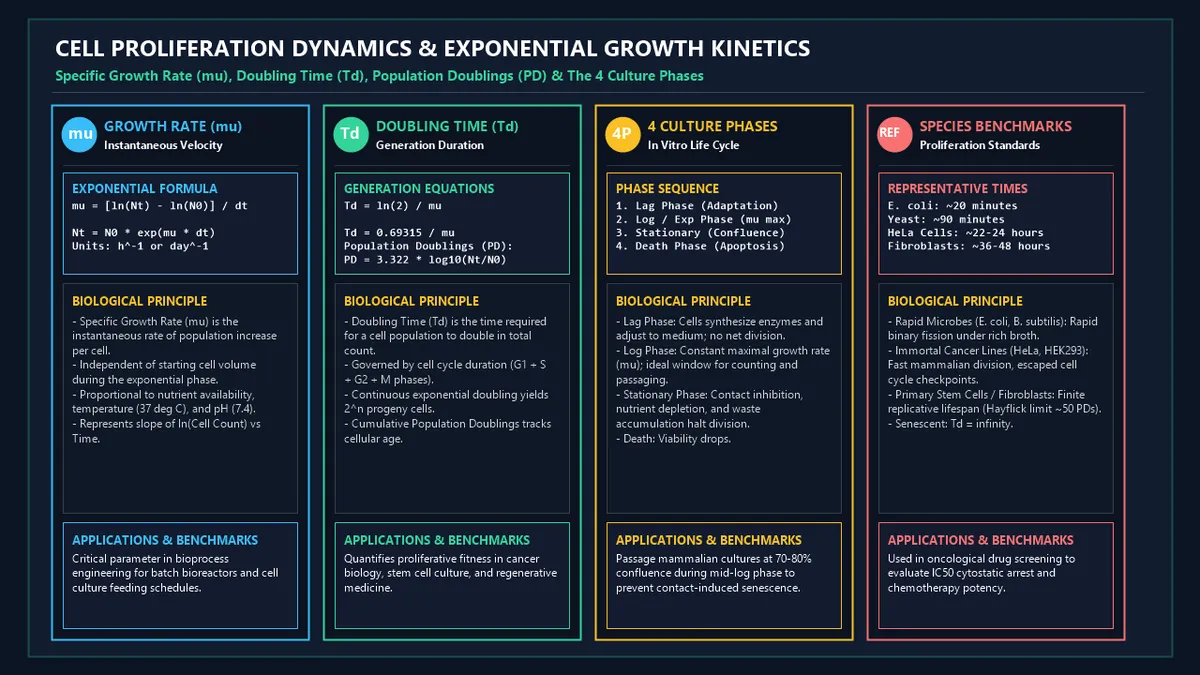
flowchart TD
    DOUBLING_SPECTRUM["Cellular Doubling Time (Td) Across Biological Systems"]

    DOUBLING_SPECTRUM --> ULTRA["⚡ Ultra-Rapid Microbes (Td < 2 Hours)
• Escherichia coli (~20 min)
• Bacillus subtilis (~30 min)
• Saccharomyces cerevisiae (~90 min)"]
    DOUBLING_SPECTRUM --> CANCER["🔬 Immortalized Mammalian & Cancer Lines (Td: 18 - 26 Hours)
• CHO-K1 Bioreactor Lines (~20 - 24 h)
• HeLa Cervical Cancer (~22 h)
• HEK293 Human Embryonic Kidney (~24 h)"]
    DOUBLING_SPECTRUM --> PRIMARY["🌿 Primary Human Somatic Cells (Td: 30 - 60 Hours)
• Human Dermal Fibroblasts (~32 - 40 h)
• Mesenchymal Stem Cells (~36 - 48 h)
• Endothelial Cells (~40 - 55 h)"]
    DOUBLING_SPECTRUM --> SENESCENCE["🛑 Arrested / Senescent (Td > 100 Hours to Infinity)
• Hayflick Replicative Senescence (P > 45)
• Differentiated Post-Mitotic Neurons & Cardiomyocytes"]
8. Comparative & Standards Tables
8.1 Reference Doubling Times Across Common Cell Types
| Cell Line / Organism | Biological Origin | Culture Type | Typical Doubling Time () | Optimal Splitting Confluence |
|---|---|---|---|---|
| Escherichia coli | Bacterium | Suspension Broth | Mid-log () | |
| Saccharomyces cerevisiae | Yeast | Suspension Broth | Mid-log () | |
| CHO-K1 | Chinese Hamster Ovary | Suspension / Adherent | ||
| HeLa | Human Cervical Carcinoma | Adherent Monolayer | ||
| HEK293 | Human Embryonic Kidney | Adherent / Suspension | 80% | |
| Jurkat | Human T-Lymphocyte | Suspension | ||
| Human Dermal Fibroblasts | Primary Dermis (P5) | Adherent Primary | (Never ) | |
| Human Bone Marrow MSCs | Primary Mesenchymal | Adherent Stem Cell | 70% (Prevent differentiation) | |
| Senescent Fibroblasts | Late Passage Primary | Flattened Monolayer | Irreversible arrest |
8.2 Seeding Density Guidelines for Standard Tissue Culture Plasticware
| Culture Vessel | Surface Area () | Recommended Seeding Density () | Confluent Yield at 100% () | Working Medium Volume |
|---|---|---|---|---|
| 96-Well Plate | ||||
| 24-Well Plate | ||||
| 6-Well Plate | ||||
| T-25 Flask | ||||
| T-75 Flask | ||||
| T-175 Flask |
9. Practical Real-World Applications
Example 1: In Vitro Oncology Drug Screening ( Cytostasis)
A cancer research team tests a novel CDK4/6 cell cycle inhibitor against a breast adenocarcinoma line.
- Control untreated cells show ().
- Drug-treated cells at concentration display (, ).
- Confirming cytostatic arrest without inducing immediate necrosis.
Example 2: CAR-T Cell Immunotherapy Manufacturing
Patient-derived autologous T-cells are genetically modified with a Chimeric Antigen Receptor () and expanded in a closed rocking bioreactor. Technicians track cumulative population doublings () to ensure cells achieve the target dose of within while maintaining a young, non-exhausted central memory phenotype ().
Example 3: Detecting Latent Mycoplasma Contamination
A stable HEK293 culture that consistently doubled every suddenly slows to with decreased media acidification. The growth rate drop prompts a PCR mycoplasma screen, uncovering contamination before master cell bank contamination occurred.
10. In-Depth Case Studies
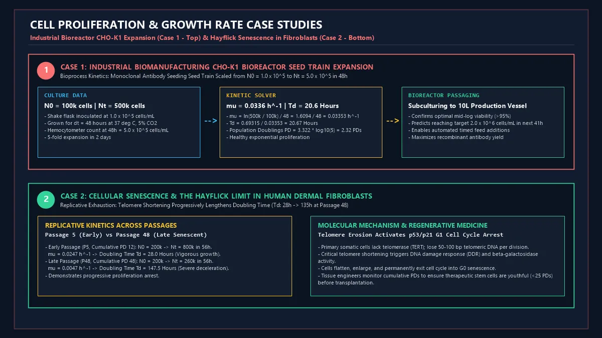
Case Study 1: Industrial Biomanufacturing CHO-K1 Bioreactor Seed Train Expansion
- Process Objective: Scale an industrial CHO-K1 clone producing a therapeutic monoclonal antibody () from shake flasks into a seed bioreactor.
- Experimental Parameters:- Initial Inoculum: ($100,000$)- Duration: at- Final Viable Density: ($500,000$)
- Kinetic Calculation:
- Bioprocess Optimization:- Knowing , engineers calculate that reaching the required bioreactor seeding density of will take exactly:- The automated feed program is scheduled to initiate at exactly , ensuring zero nutrient depletion and maximizing antibody expression titers.
Case Study 2: Cellular Senescence & The Hayflick Limit in Human Dermal Fibroblasts
- Clinical Scenario: A regenerative medicine lab produces autologous dermal fibroblast sheets for severe burn wound grafting.
- Passage-Dependent Proliferation Tracking:- Early Passage (P5, CPD 12): .- Late Passage (P48, CPD 48): .
- Biochemical Findings:- Late-passage cells show positivity, elevated and expression, and critically shortened telomeres ().
- Quality Control Decision:- Imposes a strict release criterion: All clinical cell therapy batches must have cumulative population doublings () to guarantee robust grafting potential.
11. Advantages of Mathematical Growth Rate Modeling
- Eliminates Subjective Visual Guesswork: Replaces estimated "confluence percentages" with rigorous numerical cell density () and doubling times.
- Standardizes Seed Train Schedules: Enables precise prediction of harvest hours, media exchanges, and bioreactor transfer windows.
- Ensures Batch-to-Batch Quality Control: Flags phenotypic instability, genetic mutation, contamination, or media degradation immediately.
- Distinguishes Passage Number from Biological Age: Tracks cumulative population doublings (), which reflects true telomeric aging far more accurately than arbitrary passage counts.
12. Methodological Complexities & Artifacts
- Counting Errors from Cellular Clumping: Clumped suspension cells or poorly trypsinized monolayers skew hemocytometer and automated optical counter data, leading to severe undercounting of .
- Lag Phase Distortion: Calculating doubling time immediately after thawing or heavy splitting introduces an artificial lag phase, falsely inflating the measured .
- Serum Lot-to-Lot Inconsistency: Variations in growth factor concentrations across Fetal Bovine Serum () batches can alter mammalian by .
13. Common Mistakes to Avoid
1. Calculating Doubling Time Outside the Exponential Log Phase:
Measuring cell counts during the initial lag phase or when the culture has reached 100% saturation confluence produces mathematically meaningless, falsely elevated doubling times.
2. Confusing Passage Number () with Population Doublings ():
A culture split at $1:2$ undergoes , while a culture split at $1:10$ undergoes . Tracking passage number alone masks actual cellular age.
3. Ignoring Non-Viable Dead Cells:
Failing to utilize viability exclusion dyes (Trypan Blue, Propidium Iodide) leads to total cell counts that mask culture death phase collapse.
12. Frequently Asked Questions (FAQ)
What is the difference between doubling time and growth rate?
Specific Growth Rate () is the instantaneous rate of cellular division per unit of time (e.g., ), while Doubling Time () is the total time required for the population to double (). They are inverse mathematical reflections of the same kinetic process.
Why must doubling time be measured only during the log phase?
During the lag phase, cells are adapting without dividing (). In the stationary phase, division halts due to contact inhibition and nutrient exhaustion (). Only the logarithmic phase exhibits constant, uninhibited exponential growth ().
How is Population Doubling () calculated?
Population doublings are calculated using the base-2 logarithmic formula: For example, a () equals .
What is the Hayflick Limit?
The Hayflick Limit is the finite number of times a normal primary human somatic cell population can divide (typically ) before telomere shortening triggers irreversible replicative senescence.
Why do cancer cells have indefinite doubling capacity?
Cancer cells and immortalized lines (such as HeLa or CHO) constitutively express telomerase reverse transcriptase () or utilize alternative lengthening of telomeres (), preventing telomere erosion and bypassing the Hayflick limit.
What causes doubling time to suddenly increase in a culture?
Sudden doubling time prolongation is commonly caused by mycoplasma or viral contamination, nutrient depletion, toxic lactate/ammonia accumulation, sub-optimal incubator temperature/, over-trypsinization damage, or senescence.
How does split ratio impact population doublings?
- A yields ().
- A yields ().
- A yields ().
15. Expert Tips for Cell Biologists, Bioprocess Engineers & Tissue Culturists
- Subculture at 70–80% Confluence: Never allow adherent mammalian cultures to reach 100% contact-inhibited confluence, as high cell density triggers contact-induced senescence and downregulates proliferative stemness markers.
- Maintain a Cumulative Population Doubling (CPD) Log: Document initial seeding, final harvest, and calculated at every single passage to monitor cellular drift and replicative fitness.
- Use Live-Cell Impedance or Automated Imaging: For critical kinetic studies, employ continuous live-cell monitoring systems (e.g., IncuCyte or xCELLigence) to generate continuous real-time growth curves without disturbing incubator equilibrium.
16. Summary Checklist
- ✔ Record Seeding Inoculum (): Count viable cells at time via trypan blue exclusion.
- ✔ Record Harvest Yield (): Harvest and quantify viable cells at elapsed time $\Delta t$.
- ✔ Verify Logarithmic Growth: Ensure cell density remained between 20% and 80% confluence.
- ✔ Calculate Specific Growth Rate: Solve .
- ✔ Compute Doubling Time: Solve .
- ✔ Update Cumulative Population Doublings: Add to cumulative cell history.
- ✔ Screen for Deviations: Compare against reference standards ( for immortalized lines).
Additional Technical Guidelines & Measurement Standards
When conducting calculations for Cell Doubling Time & Growth Rate Solver, maintaining quantitative precision and verifying input parameter boundaries is essential for reliable scenario evaluation. Always verify that raw numerical inputs are measured using standardized instrumentation, and double-check unit conversions prior to applying outputs in commercial, industrial, or academic projects.
For quantitative unit conversions and scientific calculations, always maintain at least four decimal places of precision during intermediate arithmetic stages before rounding final results. When preparing technical reports, laboratory documentation, or financial forecasts, cross-verify all output variables against established international measurement standards (such as SI, NIST, and ISO metric benchmarks) to guarantee consistent analytical rigor across all computational workflows.
MathsLover.com delivers this interactive solver 100% free of charge to foster global mathematical literacy, educational accessibility, and data-driven problem solving across scientific, technical, and academic communities worldwide.