💡 Direct Answer & Executive Summary (Hardy-Weinberg Allele Frequency Solver)
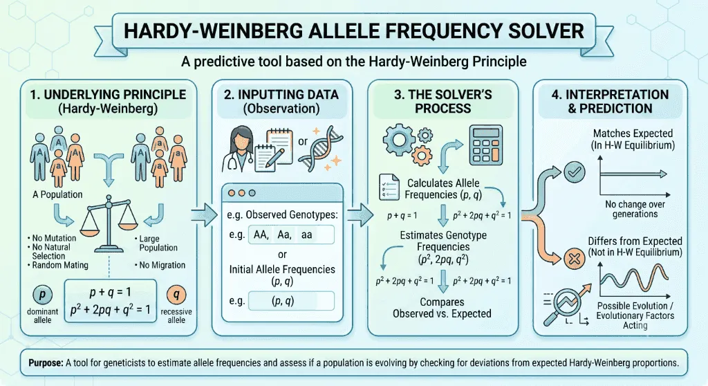
Definition: Calculate dominant and recessive allele frequencies (p, q), genotype population frequencies (p², 2pq, q²), and carrier headcount in population genetics according to the Hardy-Weinberg equilibrium principle.
Governing Math Formula: Hardy-Weinberg Principle: Allele Frequencies: p + q = 1. Genotypic Expansion: p² (Homozygous Dominant) + 2pq (Heterozygous Carrier) + q² (Homozygous Recessive) = 1. Given q²: q = √q², p = 1 - q.
Target Applications: Provides real-time quantitative solutions in Biology for students, engineers, researchers, and finance professionals.
Hardy-Weinberg Allele Frequency Solver: Population Genetics & Carrier Frequency Guide
1. Introduction
How do geneticists determine the carrier frequency of rare genetic diseases in human populations? Why don't dominant biological traits (such as brown eyes or polydactyly) continually increase in frequency until they completely eliminate recessive traits?
Formulated independently in 1908 by English mathematician G. H. Hardy and German physician Wilhelm Weinberg, the Hardy-Weinberg Principle (HWP) is the foundational mathematical theorem of modern population genetics and evolutionary biology.
The theorem states that in a large, randomly mating population free from evolutionary evolutionary forces, both allele and genotype frequencies remain constant (in equilibrium) from generation to generation.
graph LR
    SAMPLE_IN["📊 Population Data
Recessive Phenotype q² = 0.09 (9%)
Total Population N = 10,000"] --> HW_ENG["🧮 Hardy-Weinberg Engine
q = √q² = 0.30
p = 1 - q = 0.70
2pq = 2(0.70)(0.30) = 0.42"]
    HW_ENG --> ALLELE_OUT["🧬 Alleles: Dominant p = 70.0% | Recessive q = 30.0%"]
    HW_ENG --> CARRIER_OUT["🩺 Carriers (2pq): 42.0% (4,200 Carriers in N=10k)"]
    HW_ENG --> HOMO_DOM["🔬 Homozygous Dominant (p²): 49.0% (4,900 Individuals)"]
    HW_ENG --> HOMO_REC["🔬 Homozygous Recessive (q²): 9.0% (900 Affected)"]
Mastering Hardy-Weinberg equations enables genetic epidemiologists, evolutionary biologists, and public health researchers to:
- Estimate the hidden asymptomatic carrier rate () for autosomal recessive diseases (Cystic Fibrosis, Sickle Cell Anemia, Phenylketonuria [PKU]).
- Test whether natural selection, genetic drift, assortative mating, or migration is driving evolution at a specific genetic locus.
- Optimize conservation genetics management for endangered species breeding programs.
2. Definitions & Mathematical Formulations
2.1 The Two Fundamental Hardy-Weinberg Equations
Consider a single gene locus with two alleles:
- = Frequency of the Dominant Allele () in the gene pool ().
- = Frequency of the Recessive Allele () in the gene pool ().
1. Allele Frequency Equation
Because there are only two alleles at this locus, their combined frequencies must sum to unity (100%):
2. Genotype Frequency Equation (Binomial Expansion)
Squaring both sides of the allele frequency equation describes the expected diploid genotype frequencies among offspring:
Where:
- = Frequency of Homozygous Dominant individuals ().
- = Frequency of Heterozygous Carrier individuals ().
- = Frequency of Homozygous Recessive individuals () (Phenotypically expressed / Affected).
flowchart TD
    START["Input Known Parameter (e.g. Recessive Disease Incidence q²)"] --> STEP1["Step 1: Calculate Recessive Allele Frequency q = √q²"]
    STEP1 --> STEP2["Step 2: Calculate Dominant Allele Frequency p = 1 - q"]
    STEP2 --> STEP3["Step 3: Calculate Heterozygous Carrier Frequency 2pq = 2 × p × q"]
    STEP3 --> STEP4["Step 4: Calculate Homozygous Dominant Frequency p² = p × p"]
    STEP4 --> STEP5["Step 5: Project Headcount in Total Population N (p²·N, 2pq·N, q²·N)"]
    STEP5 --> DISPLAY["Display Complete Allele & Genotype Population Distribution"]
3. The 5 Foundational Assumptions of Hardy-Weinberg Equilibrium
For a population to remain in Hardy-Weinberg equilibrium, five strict biological conditions must be satisfied:
graph TD
    ASSUMP["🏛️ 5 Conditions for Hardy-Weinberg Equilibrium"]
    ASSUMP --> C1["1. Infinitely Large Population
Prevents sampling error and genetic drift"]
    ASSUMP --> C2["2. Completely Random Mating (Panmixia)
No sexual selection, assortative mating, or inbreeding"]
    ASSUMP --> C3["3. No Mutation
No net biochemical conversion of A ↔ a alleles"]
    ASSUMP --> C4["4. No Gene Flow / Migration
Closed population with zero immigration or emigration"]
    ASSUMP --> C5["5. No Natural Selection
All genotypes (AA, Aa, aa) have equal reproductive fitness (w = 1)"]If a real-world population deviates significantly from (as determined by a Chi-Square goodness-of-fit test), at least one of these five evolutionary forces is actively operating.
4. Master Clinical Genetics Case Study: Cystic Fibrosis
Cystic Fibrosis (CF) is an autosomal recessive genetic disease affecting the CFTR chloride channel. In populations of Northern European descent, the incidence of newborns born with Cystic Fibrosis is approximately live births.
Step-by-Step Mathematical Calculation:
- Identify the Recessive Phenotype Frequency ():
- Calculate the Recessive Allele Frequency ():
- Calculate the Dominant Allele Frequency ():
- Calculate the Heterozygous Carrier Frequency ():
- Calculate the Homozygous Dominant Frequency ():
Clinical Population Takeaway:
In a city of $1,000,000$ people:
- Affected individuals (): .
- Healthy non-carriers (): .
- Asymptomatic carriers (): ( more common than affected individuals!).
5. Master Population Genetics Frequency Table
| Recessive Incidence () | Recessive Allele () | Dominant Allele () | Carrier Frequency () | Carrier Ratio in Population | Example Condition |
|---|---|---|---|---|---|
| ($0.01$) | $0.1000$ | $0.9000$ | 18.00% | Sickle Cell Trait (West Africa) | |
| ($0.0025$) | $0.0500$ | $0.9500$ | 9.50% | Beta Thalassemia (Mediterranean) | |
| ($0.0004$) | $0.0200$ | $0.9800$ | 3.92% | Cystic Fibrosis (Caucasian) | |
| ($0.0001$) | $0.0100$ | $0.9900$ | 1.98% | Phenylketonuria (PKU) | |
| () | $0.00316$ | $0.99684$ | 0.63% | Albinism (Oculocutaneous) |
6. Frequently Asked Questions (FAQ)
What is the difference between and ?
- is the frequency of the single dominant allele () in the gamete gene pool.
- is the proportion of diploid individuals in the population who possess the homozygous dominant genotype ().
Why are recessive disease carriers so much more common than affected individuals?
Because when is small (e.g. $0.01$), squaring it () produces a very small number, whereas is . Most rare recessive alleles are hidden in heterozygous carriers.
What is genetic drift?
Genetic drift is the random fluctuation in allele frequencies from generation to generation due to chance sampling events. It exerts its strongest evolutionary effect in small populations.
7. Summary Checklist
- ✔ Select Input Parameter: Choose (disease frequency), , , or observed count.
- ✔ Enter Value & Population Size: Input parameters (e.g. $0.09$ in ).
- ✔ Review Allele Frequencies: Inspect and .
- ✔ Inspect Carrier Rate (): Calculate total carrier headcount.
- ✔ Verify Equilibrium Proof: Ensure .
Additional Technical Guidelines & Measurement Standards
When conducting calculations for Hardy-Weinberg Allele Frequency Solver, maintaining quantitative precision and verifying input parameter boundaries is essential for reliable scenario evaluation. Always verify that raw numerical inputs are measured using standardized instrumentation, and double-check unit conversions prior to applying outputs in commercial, industrial, or academic projects.
For quantitative unit conversions and scientific calculations, always maintain at least four decimal places of precision during intermediate arithmetic stages before rounding final results. When preparing technical reports, laboratory documentation, or financial forecasts, cross-verify all output variables against established international measurement standards (such as SI, NIST, and ISO metric benchmarks) to guarantee consistent analytical rigor across all computational workflows.
MathsLover.com delivers this interactive solver 100% free of charge to foster global mathematical literacy, educational accessibility, and data-driven problem solving across scientific, technical, and academic communities worldwide.